4. Linearized Wave Theory

Maija Benitz

4. Linearized Wave Theory

The first section of this chapter mentioned several different types of ocean waves, and we know from observation that the surface of the ocean is comprised of waves of many heights, lengths, and speeds. However, to develop a solid basis for understanding and modeling these complex wave fields, we need to start with a simpler form of wave. Here, we explore linear wave theory, or Airy wave theory, which provides a mathematical description of gravity waves traveling at the ocean surface. This theory will serve as the foundation for constructing more complex wave models.

Assumptions

In the previous section, we encountered a non-linear partial differential equation in the dynamic interfacial boundary condition—an obstacle that complicates the analytical solution of wave equations. To address this, we will introduce a series of simplifying assumptions that allow us to derive an analytically solvable model. While these assumptions may seem restrictive, they lead to a manageable set of equations that can reasonably describe the behavior of simple water waves. Later, we’ll build upon this basic solution to model more complex wave systems.

Our assumptions for linear wave theory (or Airy wave theory) include that:

Two-dimensional wave motion: Waves are assumed to propagate in a single horizontal direction (x-direction) while oscillating vertically (z-direction).
Progressive gravity waves: The waves are driven by gravity as the restoring force.
Constant wave properties: The wave period, height, and wavelength remain constant throughout the wave motion.
Uniform ocean floor: Waves are assumed to travel over a smooth, horizontal bed, meaning the seafloor is neither sloped nor rough.
Inviscid flow: The flow has no viscosity, allowing us to neglect viscous effects.
Incompressible fluid: The divergence of velocity is zero, meaning the fluid density does not change.
Irrotational flow: The flow has no vorticity, ensuring that the water particles do not rotate as the wave passes.
Homogeneous properties: There are no temperature or salinity gradients affecting wave motion.
Small wave height relative to wavelength and water depth: The wave height is assumed to be much smaller than both the wavelength and water depth, allowing us to treat the wave as “small amplitude.”

These assumptions simplify the governing equations, leading to a linearized model for wave motion that provides useful insights into the behavior of ocean waves. By understanding this foundational theory, we can later apply modifications and relaxations to these assumptions, thereby developing models that better reflect the complexities of natural ocean waves.

Fundamental Equations

The derivation of linearized wave theory begins with the Laplace equation (discussed in Chapter 6) where $\phi$ is the velocity potential .

$\nabla^2 \phi = 0$

Recall that $\nabla^2$ is the Laplace operator, which if it acts on $f$ , is the same as $\nabla \cdot \nabla f$ .

Three boundary conditions follow, beginning with an equation to describe the sea bed (or seafloor).

$\frac{\partial \phi}{\partial z} = 0$ at $z = -h$

This statement says that the partial derivative of the velocity potential in the vertical (z-direction) is equal to zero at the sea floor, which is defined where z equals -h.

Next, the kinematic boundary condition (KBC), as discussed in the previous section, is given by,

$\frac{\partial \eta}{\partial t} +\frac{\partial \phi}{\partial x} \frac{\partial \eta}{\partial x} =\frac{\partial \phi}{\partial z}$

where $\eta$ is the free surface. The second term in the KBC is non-linear due to the multiplication of terms. We can assume the partial derivatives to be small (less than one), such that their product is even smaller. Therefore, we will neglect this non-linear term. We now arrive at a KBC that is linear and defined at the surface of the ocean where z equals $\eta$ .

$\frac{\partial \eta}{\partial t} =\frac{\partial \phi}{\partial z}$ at $z = \eta$

Finally, we’ll work towards also linearizing the dynamic boundary condition (DBC), defined previously as

$\frac{\partial \phi}{\partial t} + \frac{1}{2}[ (\frac{\partial \phi}{\partial x})^2 + (\frac{\partial \phi}{\partial y})^2 ] + g \eta = f(t)$

by again neglecting any non-linear terms, resulting in,

$\frac{\partial \phi}{\partial t} + g \eta = 0$ at $z = \eta$

Airy Waves

By separation of variables, we arrive at expressions for the velocity potential, $\phi$ , and surface elevation, $\eta$ .

$\phi(x,z,t) = \frac{gH}{2kc} \frac{cosh[k(z+h)]}{cosh(kh)} sin[k(x-ct)]$

$\eta(x,t) = \frac{H}{2} cos(kx -\omega t + \theta)$

where g is gravity, H is wave height, k is wavenumber, c is wave speed (aka celerity), h is water depth, $\omega$ is the angular frequency of the wave, and $\theta$ is the phase angle. These equations are the solutions to linear (small amplitude) wave theory.

Solutions for the velocity potential must satisfy the “dispersion relation”, which uniquely relates the wave number to the wave frequency for a given water depth. It a result of the KBC given above.

$\omega^2 = gk\text{ } tanh(kh)$

**Figure 7.4.1** Sine wave with annotations (By Kraaiennest (Own work) [CC BY-SA 3.0], via Wikimedia Commons).

Several new variables were introduced in this section, so it bears defining them and relating them to one another. First, the wavenumber, k, is defined at the ratio of $2 \pi$ over the wavelength $\lambda$ .

$k = \frac{2 \pi}{\lambda}$

The wave frequency, $\omega$ , can be computed as either the ratio of $2 \pi$ over the wave period $T$ , or the product of $2 \pi$ and the linear wave frequency f.

$\omega = \frac{2 \pi}{T} = 2 \pi f$

Finally, the wave speed (aka celerity) is equivalent to the two ratios below,

$c = \frac{\omega}{k} = \frac{\lambda}{T}$

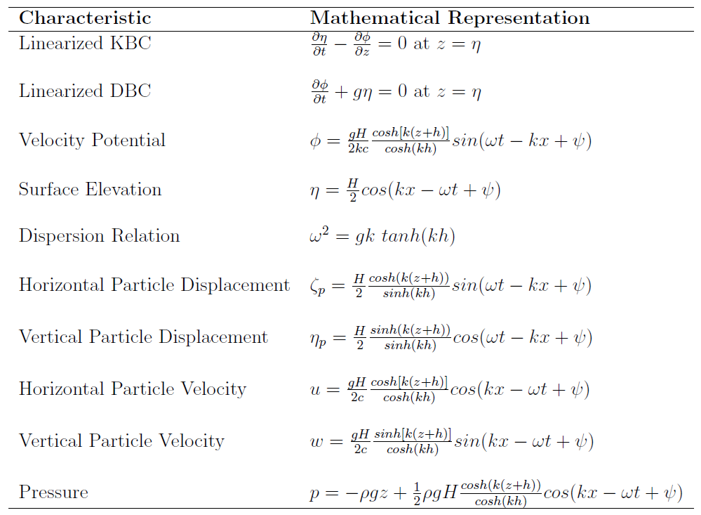
Summary of Equations

Expressions can also be derived for water particle displacements and velocities. The solutions to those equations and the ones previously discussed for linearized wave theory are summarized in Table 7.4.1 below.

**Table 7.4.1** Summary of Linearized Wave Theory equations.

Visualizing the Flow

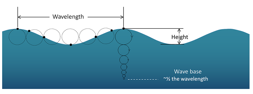
Although waves can travel over great distances, the water itself shows little horizontal movement; it is the energy of the wave that is being transmitted, not the water. Instead, the water particles move in circular orbits, with the size of the orbit equal to the wave height (Figure 7.4.2). This orbital motion occurs because water waves contain components of both longitudinal (side to side) and transverse (up and down) waves, leading to circular motion. As a wave passes, water moves forwards and up over the wave crests, then down and backwards into the troughs. In Airy wave theory the particle paths are closed. This is evident if you have ever watched an object such as a seabird floating at the surface. The bird bobs up and down as the wave pass underneath it; it does not get carried horizontally by a single wave crest.

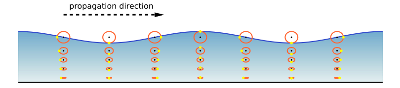
**Figure 7.4.2** Orbital motion under gravity surface waves (By Kraaiennest (Own work) [CC BY-SA 3.0], via Wikimedia Commons).

The circular orbital motion declines with depth as the wave has less impact on deeper water and the diameter of the circles is reduced. Eventually at some depth there is no more circular movement and the water is unaffected by surface wave action. This depth is the wave base and is equivalent to half of the wavelength (Figure 7.4.3). Since most ocean waves have wavelengths of less than a few hundred meters, most of the deeper ocean is unaffected by surface waves, so even in the strongest storms marine life or submarines can avoid heavy waves by submerging below the wave base.

**Figure 7.4.3** Orbital motion of water within a wave, extending down to the wave base at a depth of half of the wavelength (Modified by Paul Webb from Steven Earle, “Physical Geology”).

License

Icon for the Creative Commons Attribution-NonCommercial-ShareAlike 4.0 International License