6. Non-linear Water Waves

Maija Benitz

6. Non-linear Water Waves

Stokes Waves

In Section 4, we introduced Airy wave theory, which applies linearized boundary conditions to find solutions to the Laplace equation. It turns out that solutions for the velocity potential, $\phi$ , and the free surface elevation, $\eta$ , can also be found via a Taylor series expansion and perturbation analysis, which result in Stokes’ wave theory. Though the derivation falls outside of the scope of this text, the results and their ramifications do not.

Named after Sir George Gabriel Stokes, these waves are correctly referred to as Stokes waves, not “Stoke’s waves.” The plural “s” is part of Stokes’ name, making the distinction a matter of both punctuation and accuracy.

The free surface elevation of a Stokes wave is given generally by,

$\eta = \sum_{n=1}^{\infty} A_n \cos[n(x-ct)]$

where we can sum any number of terms from 1 to $\infty$ , to give increasingly higher order treatments of surface gravity waves. Each term is comprised of a cosine, so Stokes waves are sinusoidal, similar to Airy waves but with the potential for added accuracy.

1st Order Stokes Waves

For a 1st Order Stokes wave, only one term is included in the sum:

$\eta = A \cos(kx-\omega t + \theta)$

where where A is amplitude, k is wavenumber, x is the horizontal direction, $\omega$ is wave frequency, and $\theta$ is the phase angle.

2nd Order Stokes Waves

For a 2nd Order Stokes wave, we sum two terms:

$\eta = A \cos(kx-\omega t + \theta) +\frac{H^2}{2L} \frac{cosh(kh)(2+cosh(2kh))}{sinh^3(kh)} \cos(kx-\omega t + \theta)$

where H is the wave height (distance from trough to crest) as opposed to wave amplitude A (distance from still water line to crest). If you squint at the equation above you will see that it is just two cosine terms added together, where each term has a unique coefficient in front. The first term is identical to the formulation for a 1st Order Stokes wave. The second term, which makes this a 2nd Order formulation, uses hyperbolic cosines (cosh) in the coefficient in front of the cosine term. The point is not to get lost in the math, but to appreciate that with each extra term a higher order of accuracy is given to the solution, making it a better mathematical description of a surface gravity wave. Often the addition of the 2nd Order term is sufficiently accurate for our engineering applications, such that we need not worry about coming up with a 17th order formulation, or really even a 3rd Order.

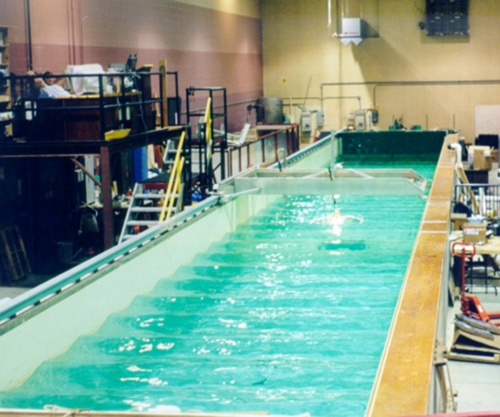
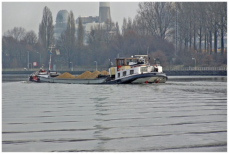
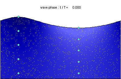
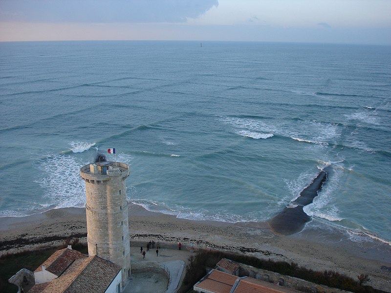
Figure 7.6.1 shows regularly repeating Stokes waves produced in a wave tank. And while is rare to observe perfectly repeating Stokes waves — those with a single amplitude and single wavelength — in the wild, sometimes with the right constraints and conditions it does occur, as shown in Figure 7.6.2.

**Figure 7.6.1** Model testing with periodic waves at the Wave/Tow Tank of the Jere A. Chase Ocean Engineering Laboratory, University of New Hampshire. (NOAA, public domain, via Wikimedia Commons).

**Figure 7.6.2** Stokes waves in the wild(ish). (Photo by digicla [CC BY 2.0], via Wikimedia Commons).

Differences Between Airy and Stokes Waves

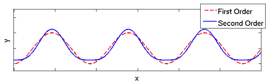
Stokes waves have sharper crests and shallower troughs than Airy waves, offering a closer match to real surface gravity waves (as shown in Figure 7.6.3).

**Figure 7.6.3** Visualization of 1st Order (linear) and 2nd Order Stokes waves, recreated from Benitz, M.A. “Simulating the Hydrodynamics of Offshore Floating Wind Turbine Platforms in a Finite Volume Framework.” (2016). https://scholarworks.umass.edu/dissertations_2/620/.

While Airy wave theory describes particle paths as closed circles or ellipses. Stokes wave theory also shows that in non-linear waves, water particles travel in unclosed paths, a phenomenon known as Stokes drift, shown in Figure 7.6.4.

**Figure 7.6.4** Animation showing the orbital motion of particles in a surface wave (By Kraaiennest (Own work) [GFDL (http://www.gnu.org/copyleft/fdl.html) or CC BY-SA 4.0], via Wikimedia Commons).

Cnoidal Waves

Cnoidal waves are used to model ocean swells—waves with long wavelengths and shallow troughs between steep crests. Named after the Jacobi elliptic function cn, cnoidal waves are periodic, similar to trigonometric functions like sine and cosine.

The Korteweg-deVries (KdV) equation is a partial differential equation that describes waves traveling on shallow water. The cnoidal wave, a solution of the KdV equation, is given by

$\eta(x,t) = \eta_2 + H cn^2 \left ( \frac{x-ct}{\Delta} \arrowvert m \right )$

where $\eta_2$ is the trough elevation, H is the wave height, c is the phase speed and $cn$ is the Jacobi elliptic function.

Figure 7.6.5 shows ocean swell travelling in one direction and Figure 7.6.6 shows the interference pattern of two crossing swells. Cnoidal waves could be used to model both cases.

**Figure 7.6.5** Periodic waves in shallow water. The original caption read: “As they near shallow water close to the coast of Panama, huge deep-sea waves, relics of a recent storm, are transformed into waves that have crests, but little or no troughs. A light breeze is blowing diagonally across the larger waves to produce a cross-chop. Three Army bombers, escorted by a training ship, are proceeding from Albrook Field, Canal Zone, to David, Panama.” (in: National Geographic 63 (1933).) (Public Domain, via Wikimedia Commons).

**Figure 7.6.6** Cross swell. Photo taken from Phares des Baleines (Lighthouse of the Whales) on Île de Ré. (Photo by Michel Griffon [CC BY 3.0], via Wikimedia Commons).

Solitary Waves (Solitons)

Solitary waves were first documented in 1834 by John Scott Russell, who observed a single wave progressing within a canal, caused by a boat that came to a sudden stop. These ways have since been recreated in wave tanks, and on rare occasions observed in the “wild” (quotes to allow canals to be a wild place). The term soliton was coined in 1965 by two American physicists. These waves are characterized by having a single peak that travels at wave speed,

$c = \sqrt{g(H+h)}$

The surface of a solitary wave is given by,

$\eta = \frac{H} { ( cosh( \sqrt{ \frac{3H}{ 4h^3}} (c t - \vec{x} ))^2 }$

where as before, H is the wave height, h is the water depth, g is gravity and $\vec{x}$ is the direction of the progressing wave.

Solitary waves are another solution of the KdV equation, but not the Navier-Stokes equations.

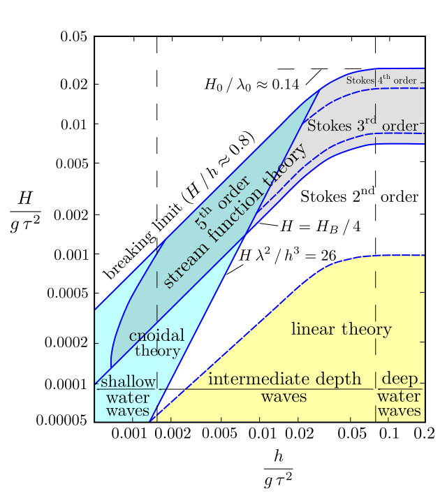
Regions of Wave Applicability

Selecting the appropriate wave model is essential for effective ocean engineering. Figure 7.6.7, adapted from Bernard Le Méhauté’s work, shows regions of validity for various wave theories, including Airy, Stokes, and cnoidal wave theories. The chart uses two parameters: wave height (H) over gravity (g) times the square of the wave period (T), and water depth. By calculating these ratios, engineers can consult the chart to determine the appropriate wave model for specific conditions.

**Figure 7.6.7.** Validity of several theories for periodic water waves, according to Le Méhauté (1976). The light-blue area is the range of validity of cnoidal wave theory; light-yellow for Airy wave theory; and the dashed blue lines demarcate the required order of Stokes’ wave theory. The light-gray shading gives the range extension by numerical approximations using fifth-order stream-function theory, for high waves (H > ¼ H_breaking). (By Kraaiennest [GFDL (http://www.gnu.org/copyleft/fdl.html) or CC BY-SA 4.0], via Wikimedia Commons).

License

Icon for the Creative Commons Attribution-NonCommercial-ShareAlike 4.0 International License