3. Boundary Conditions

Maija Benitz

3. Boundary Conditions

Completing the Governing Equations

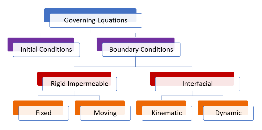
To fully define the fluid dynamics problem for water waves, we need boundary conditions to complement the fundamental equations of fluid mechanics introduced in the previous section. Since these equations describe properties that vary in both space and time, we require both spatial and temporal boundary conditions. Figure 7.3.1 summarizes the types of boundary conditions needed.

**Figure 7.3.1** The boundary conditions needed to complete the set of governing equations.

Temporal Boundary Conditions are defined by initial conditions, specifying fluid properties at the initial time. For example, at time $t = 0$ seconds, the fluid velocity in the x-direction might be given as 2 m/s, and the initial wave height as 0.65 m.

Spatial Boundary Conditions, often simply referred to as boundary conditions, define the physical limits of the problem. These include specifications like the depth of the seafloor or the locations of physical objects (e.g., boat hulls, dock pilings, shorelines). Spatial boundary conditions are further categorized into rigid impermeable and interfacial boundaries, as depicted in red in Figure 7.3.1.

Rigid Impermeable Boundary Conditions

Rigid impermeable boundaries are surfaces that are in contact with water but do not allow flow through them (impermeable) and do not deform (rigid). These can be fixed (stationary) or moving boundaries, shown in orange in Figure 7.3.1.

Fixed

Fixed Rigid Boundaries represent surfaces that are stationary, such as the seafloor, rocks, or piers. For these boundaries, the fluid velocity perpendicular to the boundary (normal velocity) must be zero, mathematically expressed as:

$u_n = \vec{u} \cdot \hat{n} = 0$

where $u_n$ is the fluid velocity normal to the object’s surface, $\vec{u}$ is the two-dimensional (or three-dimensional) velocity field surrounding the object, and $\hat{n}$ is the unit vector normal to the surface.

This can also be expressed in terms of the velocity potential, $\phi$ , (hint: potential flow theory becomes helpful here!)

$\frac{\partial \phi}{\partial n} = \nabla \phi \cdot \hat{n} = 0$

Moving

Moving Rigid Boundaries describe objects that move without deforming, like a boat hull bobbing in waves or a swimming fish. For these cases, the fluid velocity normal to the boundary equals the object’s velocity normal to its surface:

The mathematical statement for fixed bodies from above can be altered slightly to allow for motion. That is, the dot product of the fluid velocity, $\vec{u}$ , and $\hat{n}$ does not have to be strictly zero. In fact, it will be equal to the dot product of the object’s velocity, $\vec{V}$ , and $\hat{n}$ .

$u_n = \vec{u} \cdot \hat{n} = \vec{V} \cdot \hat{n}$

In terms of the velocity potential:

$\frac{\partial \phi}{\partial n} = \nabla \phi \cdot \hat{n} = \vec{V} \cdot \hat{n}$

Interfacial Boundary Conditions

Interfacial boundary conditions apply at a fluid-fluid interface, such as the air-water surface of the ocean. These boundaries can deform and require two conditions: the kinematic boundary condition and the dynamic boundary condition, shown in orange in Figure 7.3.1.

The Kinematic Boundary Condition

The Kinematic Boundary Condition relates to the motion of particles on the free surface $η\eta$ and ensures that particles remain on this interface. For ocean waves, the kinematic condition at the free surface is:

$\frac{\partial \eta}{\partial t} + \frac{\partial \phi}{\partial x} \frac{\partial \eta}{\partial x} = \frac{\partial \phi}{\partial z}$ at $z = \eta$

The Dynamic Boundary Condition

The Dynamic Boundary Condition ensures continuity of stress across the air-water interface to prevent surface rupture. Surface tension and curvature influence this condition, and although a detailed derivation is beyond this text, it results in:

$\frac{\partial \phi}{\partial t} + \frac{1}{2}[ (\frac{\partial \phi}{\partial x})^2 + (\frac{\partial \phi}{\partial y})^2 ] + g \eta = f(t)$

This non-linear boundary condition highlights the complexity of accurately describing water waves analytically. Consequently, simplifying assumptions are often necessary to make the problem more tractable, which will be our focus in the following section.

License

Icon for the Creative Commons Attribution-NonCommercial-ShareAlike 4.0 International License