
2. Icebergs
Many of the most spectacular ice formations in the ocean take the form of icebergs. Remember that the largest icebergs are not made of sea ice; they are floating pieces of glaciers that have broken off, or calved from the glacier tongue, and thus they are composed of fresh water ice.
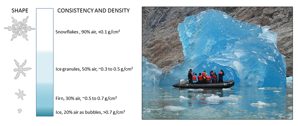
Glacial ice forms from layers of snow that accumulate over time. The weight of the accumulated layers compresses the snow into a granular form known as firn that has a higher density and less air than regular snow. As the pressure from the continued snow accumulation increases, the firn is compressed into even denser glacial ice (Figure 10.2.1). Most icebergs appear white because the ice still contains a lot of air bubbles that scatter all of the wavelengths of white light. But icebergs composed of older ice, or highly compressed ice from deep within a glacier can appear a deep shade of blue (Figure 10.2.1). This ice contains much less air, and larger, denser ice crystals that absorb the longer (red) wavelengths of light, and transmit and scatter the shorter, blue wavelengths. The longer the path that light travels through the ice, the more the long wavelengths are absorbed, and the bluer the ice appears.
Icebergs come in a wide range of sizes, from a few meters across to hundreds of kilometers long. Table 10.2.1 shows the size categories used in the North Atlantic (in the Antarctic a different scale is used, as the icebergs tend to be larger there).
Table 10.2.1 Iceberg size classifications for the North Atlantic
| Size Category | Height (m) | Length (m) |
|---|---|---|
| Growler | < 1 | < 5 |
| Bergy Bit | 1-5 | 5-15 |
| Small | 5-15 | 15-60 |
| Medium | 16-45 | 61-120 |
| Large | 46-75 | 121-200 |
| Very Large | > 75 | > 200 |
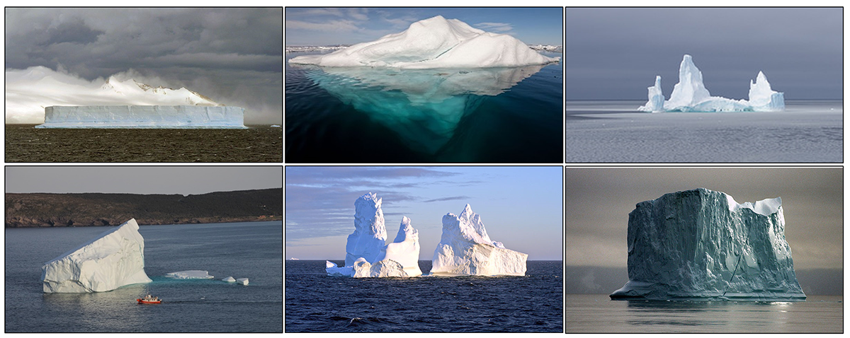
Icebergs can also be classified based on their shapes (Figure 10.2.2). The primary distinction is between tabular and non-tabular icebergs. Tabular icebergs have steep sides and a flat top, and the length is greater than five times the height. Non-tabular icebergs include any icebergs that are not tabular, and these can be further subdivided into a few categories. Domed icebergs have a rounded top, pinnacled icebergs have tall spires, and wedge icebergs have a steep face next to a more gradually sloping side. Drydock icebergs have a water-covered channel running through it, potentially large enough for boats to pass through; hence the name. Finally, blocky icebergs have a flat top and steep sides, but their length to height ratio is not as great as it is for a tabular iceberg. Regardless of the shape of an iceberg, what we see above the surface only represents about 10% of the total mass, with the rest of the ice remaining submerged (see box below).
How much of an iceberg is visible above the surface?
Archimedes’ Principle states that the upwards buoyant force of an object in water is equal to the weight of the water displaced by the object. We know that the density of an iceberg (ρi) is around 0.917 g/cm3. The weight (wi) of the iceberg is equal to its mass (mi) x the acceleration due to gravity (g), which is 9.8 m/s2. Since density = mass/volume (V), the weight of the iceberg is:
wi = ρiVig
Since the iceberg is floating at equilibrium, the weight of the iceberg (wi) is equal to the weight of the water it displaces (ww). The weight of water displaced is therefore:
ww = ρwVwg
where the density of seawater (ρw) is about 1.024 g/cm3. Now we have:
wi = ww
ρiVig = ρwVwg
so Vw = (ρi/ρw)Vi = (0.917/1.024)Vi = 0.89 Vi.
In other words, the volume of water displaced (Vw) is equal to about 89% of the volume of the iceberg (Vi). This means that 89% of the iceberg is submerged, leaving around 11% of the ice exposed above the surface.
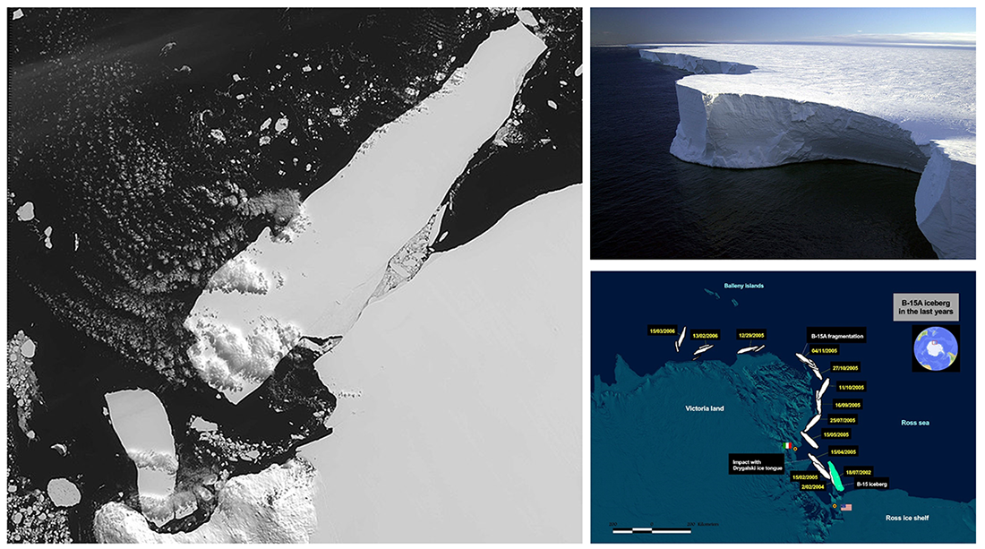
Icebergs in the Arctic tend to be smaller and more non-tabular than Antarctic icebergs, because most of them formed as irregular chunks of glaciers that calved off into the ocean, primarily around Greenland. It is estimated that the glaciers around Greenland and the Canadian Arctic calve off 300 billion cubic meters of icebergs each year. Because Antarctica has much larger ice sheets, the icebergs produced in the Southern Hemisphere are usually larger than those in the Arctic, and they tend to be more tabular in shape, as entire sections of the ice sheet break off at once. The largest iceberg ever recorded, the B-15 iceberg, broke off of the Antarctic ice sheet in 2000. It measured 295 km long and 37 km wide, giving it an area of about 11,000 square kilometers; about the size of Connecticut. Over the next few years B-15 drifted along the Antarctic coast before being broken up into smaller pieces (Figure 10.2.3).
All of these icebergs floating through the polar oceans are potentially hazardous to ship traffic, as we all know from the tragic story of the Titanic. In response to that disaster, the North Atlantic maritime nations established the International Ice Observation and Ice Patrol Service in 1914, to monitor icebergs threatening the shipping lanes. Interestingly, the original charge of the patrol also included searching for and destroying derelict ship hulls that were still floating around, as these were also a potential hazard. While the patrols were successful at destroying these abandoned ship hulls, they achieved far less success at attempting to destroy the icebergs. Eventually they gave up on iceberg destruction and focused their efforts on monitoring iceberg movements. Today, the service still operates as the International Ice Patrol, operated by the U.S. Coast Guard. Twice each day the patrol issues alerts with the position and potential tracks of existing icebergs, and the extent of the ice cover, reporting on the roughly 600 icebergs per year that intrude below 48o N latitude, the northern limit of the major shipping lines. No such iceberg patrol exists around Antarctica, as there is much less shipping traffic at those latitudes.
[latexpage]
Learning Objectives
6.5.1 Determine divergence from the formula for a given vector field.
6.5.2 Determine curl from the formula for a given vector field.
6.5.3 Use the properties of curl and divergence to determine whether a vector field is conservative.
In this section, we examine two important operations on a vector field: divergence and curl. They are important to the field of calculus for several reasons, including the use of curl and divergence to develop some higher-dimensional versions of the Fundamental Theorem of Calculus. In addition, curl and divergence appear in mathematical descriptions of fluid mechanics, electromagnetism, and elasticity theory, which are important concepts in physics and engineering. We can also apply curl and divergence to other concepts we already explored. For example, under certain conditions, a vector field is conservative if and only if its curl is zero.
In addition to defining curl and divergence, we look at some physical interpretations of them, and show their relationship to conservative and source-free vector fields.
Divergence
Divergence is an operation on a vector field that tells us how the field behaves toward or away from a point. Locally, the divergence of a vector field F in ℝ2 or ℝ3 at a particular point P is a measure of the “outflowing-ness” of the vector field at P. If F represents the velocity of a fluid, then the divergence of F at P measures the net rate of change with respect to time of the amount of fluid flowing away from P (the tendency of the fluid to flow “out of” P). In particular, if the amount of fluid flowing into P is the same as the amount flowing out, then the divergence at P is zero.
Definition
If F =$ \langle P, Q, R \rangle $ is a vector field in ℝ3and Px, Qy, and Rz all exist, then the divergence of F is defined by
Note the divergence of a vector field is not a vector field, but a scalar function. In terms of the gradient operator ∇ = 〈 $\frac{\partial}{\partial x}, \frac{\partial}{\partial y}, \frac{\partial}{\partial z}$ 〉 divergence can be written symbolically as the dot product
Note this is merely helpful notation, because the dot product of a vector of operators and a vector of functions is not meaningfully defined given our current definition of dot product.
If F=〈P, Q〉 is a vector field in ℝ2, and Px and Qy both exist, then the divergence of F is defined similarly as
div F = $P_x + Q_y$ = $\frac{\partial P}{\partial x} + \frac{\partial Q}{\partial y}$ = ∇⋅F.
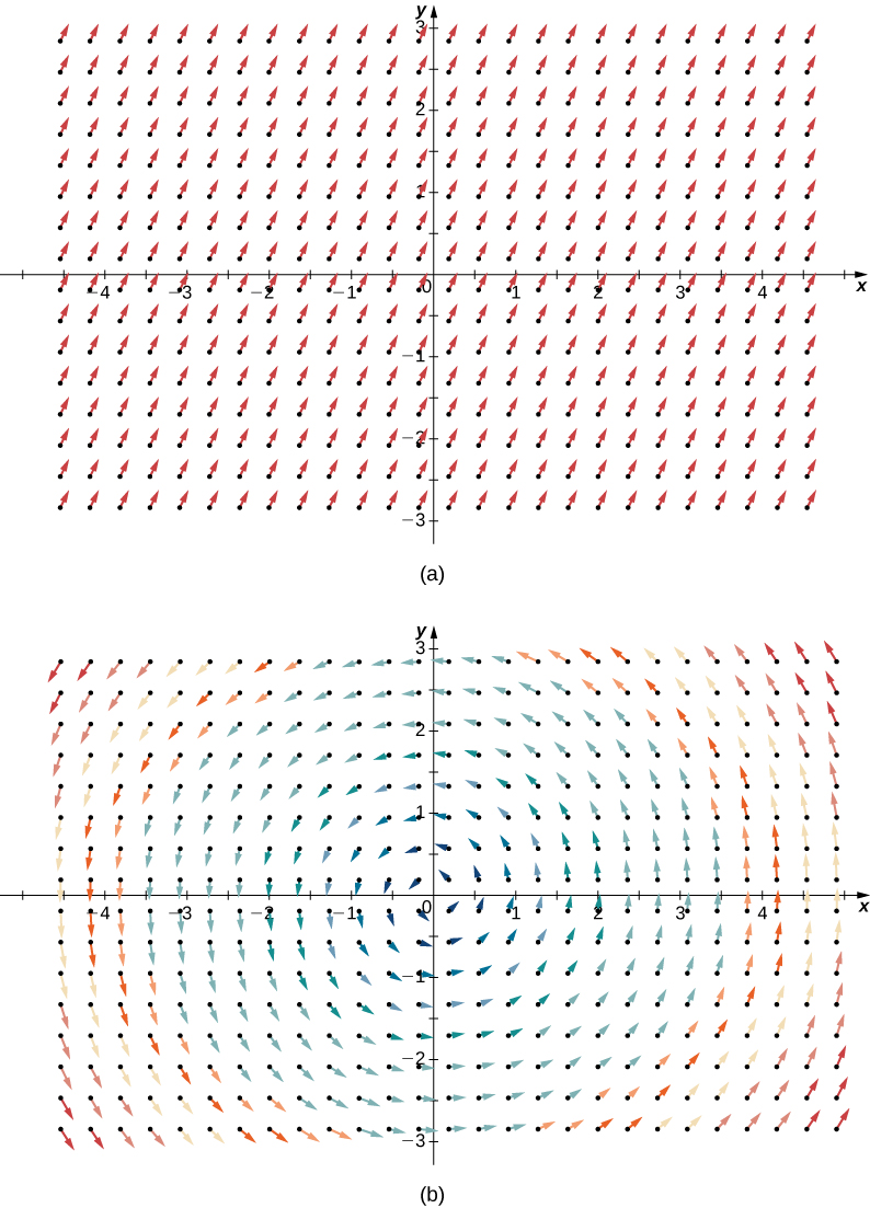
To illustrate this point, consider the two vector fields in Figure 6.50. At any particular point, the amount flowing in is the same as the amount flowing out, so at every point the “outflowing-ness” of the field is zero. Therefore, we expect the divergence of both fields to be zero, and this is indeed the case, as
div(〈1,2〉) = $\frac{\partial}{\partial x}(1) + \frac{\partial}{\partial y}(2)$
and
div(〈-y,x〉) = $\frac{\partial}{\partial x}(-y) + \frac{\partial}{\partial y}(x)$
By contrast, consider radial vector field R(x,y)=〈−x,−y〉 in Figure 6.51. At any given point, more fluid is flowing in than is flowing out, and therefore the “outgoingness” of the field is negative. We expect the divergence of this field to be negative, and this is indeed the case, as div(R) = $\frac{\partial}{\partial x}(-x) + \frac{\partial}{\partial y}(-y)$ = -2.
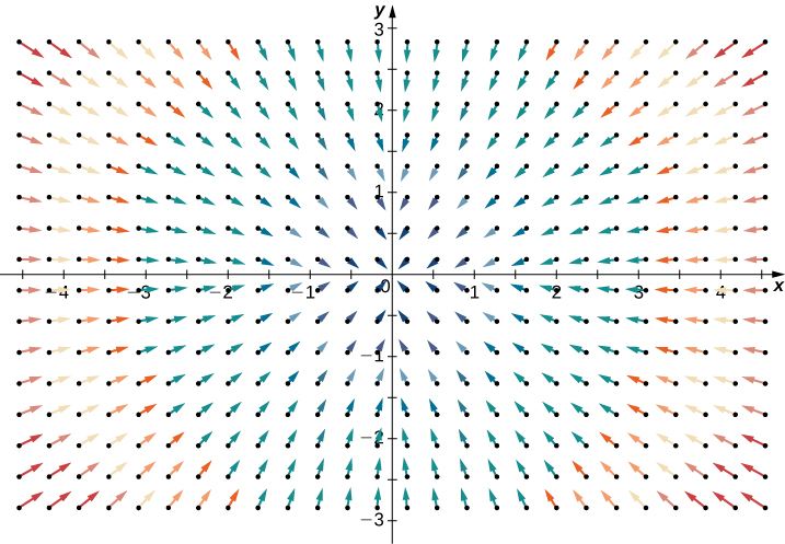
To get a global sense of what divergence is telling us, suppose that a vector field in ℝ2 represents the velocity of a fluid. Imagine taking an elastic circle (a circle with a shape that can be changed by the vector field) and dropping it into a fluid. If the circle maintains its exact area as it flows through the fluid, then the divergence is zero. This would occur for both vector fields in Figure 6.50. On the other hand, if the circle’s shape is distorted so that its area shrinks or expands, then the divergence is not zero. Imagine dropping such an elastic circle into the radial vector field in Figure 6.51 so that the center of the circle lands at point (3, 3). The circle would flow toward the origin, and as it did so the front of the circle would travel more slowly than the back, causing the circle to “scrunch” and lose area. This is how you can see a negative divergence.
Example: Calculating Divergence at a Point
If F(x,y,z)=exi+yzj-yz2k, then find the divergence of F at (0,2,-1).
Solution
The divergence of F is
$\frac{\partial}{\partial x}(e^2) + \frac{\partial}{\partial y}(yz)-\frac{\partial}{\partial z}(yz^2)$
Therefore, the divergence at (0,2,−1) is e0−1+4=4. If F represents the velocity of a fluid, then more fluid is flowing out than flowing in at point (0,2,−1).
One application for divergence is detecting whether a field is source free. Recall that a source-free field is a vector field that has a stream function; equivalently, a source-free field is a field with a flux that is zero along any closed curve. The next two theorems say that, under certain conditions, source-free vector fields are precisely the vector fields with zero divergence.
Theorem
Divergence of a Source-Free Vector Field
If F = 〈P,Q〉 is a source-free continuous vector field with differentiable component functions, then div F=0.
Proof
Since F is source free, there is a function g(x,y)with gy=P and −gx=Q. Therefore, F=〈gy,−gx〉 and div F=〈gyx−gxy〉 = 0 by Clairaut’s theorem.
□
The converse of Divergence of a Source-Free Vector Field is true on simply connected regions, but the proof is too technical to include here. Thus, we have the following theorem, which can test whether a vector field in ℝ2 is source free.
Theorem
Divergence Test for Source-Free Vector Fields
Let F=〈P,Q〉 be a continuous vector field with differentiable component functions with a domain that is simply connected. Then, div F=0 if and only if F is source free.
Example: Determining Whether a Field Is Source Free
Is field F(x,y)=〈x2y,5−xy2〉 source free?
Solution
Note the domain of F is ℝ2, which is simply connected. Furthermore, F is continuous with differentiable component functions. Therefore, we can use Divergence Test for Source-Free Vector Fields to analyze F. The divergence of F is
Therefore, F is source free by Divergence Test for Source-Free Vector Fields.
Checkpoint 6.41
Let
be a rotational field where a and b are positive constants. Is F source free?
Recall that the flux form of Green’s theorem says that
where C is a simple closed curve and D is the region enclosed by C. Since
Green’s theorem is sometimes written as
Therefore, Green’s theorem can be written in terms of divergence. If we think of divergence as a derivative of sorts, then Green’s theorem says the “derivative” of F on a region can be translated into a line integral of F along the boundary of the region. This is analogous to the Fundamental Theorem of Calculus, in which the derivative of a function
on a line segment
can be translated into a statement about
on the boundary of
Using divergence, we can see that Green’s theorem is a higher-dimensional analog of the Fundamental Theorem of Calculus.
We can use all of what we have learned in the application of divergence. Let v be a vector field modeling the velocity of a fluid. Since the divergence of v at point P measures the “outflowing-ness” of the fluid at P,
implies that more fluid is flowing out of P than flowing in. Similarly,
implies the more fluid is flowing in to P than is flowing out, and
implies the same amount of fluid is flowing in as flowing out.
Example 6.51
Determining Flow of a Fluid
Suppose
models the flow of a fluid. Is more fluid flowing into point
than flowing out?
Solution
To determine whether more fluid is flowing into
than is flowing out, we calculate the divergence of v at
To find the divergence at
substitute the point into the divergence:
Since the divergence of v at
is negative, more fluid is flowing in than flowing out (Figure 6.53).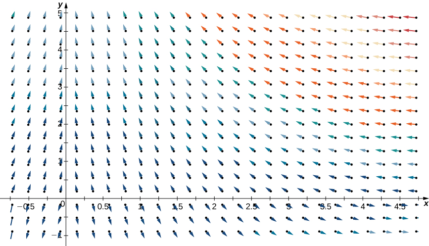
Figure 6.53 Vector field
has negative divergence at
Checkpoint 6.42
For vector field
find all points P such that the amount of fluid flowing in to P equals the amount of fluid flowing out of P.
Curl
The second operation on a vector field that we examine is the curl, which measures the extent of rotation of the field about a point. Suppose that F represents the velocity field of a fluid. Then, the curl of F at point P is a vector that measures the tendency of particles near P to rotate about the axis that points in the direction of this vector. The magnitude of the curl vector at P measures how quickly the particles rotate around this axis. In other words, the curl at a point is a measure of the vector field’s “spin” at that point. Visually, imagine placing a paddlewheel into a fluid at P, with the axis of the paddlewheel aligned with the curl vector (Figure 6.54). The curl measures the tendency of the paddlewheel to rotate.
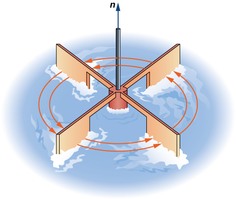
Figure 6.54 To visualize curl at a point, imagine placing a small paddlewheel into the vector field at a point.
Consider the vector fields in Figure 6.50. In part (a), the vector field is constant and there is no spin at any point. Therefore, we expect the curl of the field to be zero, and this is indeed the case. Part (b) shows a rotational field, so the field has spin. In particular, if you place a paddlewheel into a field at any point so that the axis of the wheel is perpendicular to a plane, the wheel rotates counterclockwise. Therefore, we expect the curl of the field to be nonzero, and this is indeed the case (the curl is
To see what curl is measuring globally, imagine dropping a leaf into the fluid. As the leaf moves along with the fluid flow, the curl measures the tendency of the leaf to rotate. If the curl is zero, then the leaf doesn’t rotate as it moves through the fluid.
Definition
If
is a vector field in
and
and
all exist, then the curl of F is defined by

(6.17)
Note that the curl of a vector field is a vector field, in contrast to divergence.
The definition of curl can be difficult to remember. To help with remembering, we use the notation
to stand for a “determinant” that gives the curl formula:

The determinant of this matrix is
Thus, this matrix is a way to help remember the formula for curl. Keep in mind, though, that the word determinant is used very loosely. A determinant is not really defined on a matrix with entries that are three vectors, three operators, and three functions.
If
is a vector field in
then the curl of F, by definition, is
Example 6.52
Finding the Curl of a Three-Dimensional Vector Field
Find the curl of
Solution
The curl is

Checkpoint 6.43
Find the curl of
at point
Example 6.53
Finding the Curl of a Two-Dimensional Vector Field
Find the curl of
Solution
Notice that this vector field consists of vectors that are all parallel. In fact, each vector in the field is parallel to the x-axis. This fact might lead us to the conclusion that the field has no spin and that the curl is zero. To test this theory, note that
Therefore, this vector field does have spin. To see why, imagine placing a paddlewheel at any point in the first quadrant (Figure 6.55). The larger magnitudes of the vectors at the top of the wheel cause the wheel to rotate. The wheel rotates in the clockwise (negative) direction, causing the coefficient of the curl to be negative.
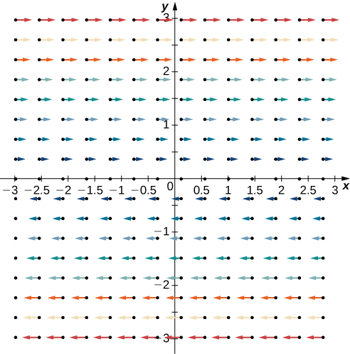
Figure 6.55 Vector field
consists of vectors that are all parallel.
Note that if
is a vector field in a plane, then
Therefore, the circulation form of Green’s theorem is sometimes written as
where C is a simple closed curve and D is the region enclosed by C. Therefore, the circulation form of Green’s theorem can be written in terms of the curl. If we think of curl as a derivative of sorts, then Green’s theorem says that the “derivative” of F on a region can be translated into a line integral of F along the boundary of the region. This is analogous to the Fundamental Theorem of Calculus, in which the derivative of a function
on line segment
can be translated into a statement about
on the boundary of
Using curl, we can see the circulation form of Green’s theorem is a higher-dimensional analog of the Fundamental Theorem of Calculus.
We can now use what we have learned about curl to show that gravitational fields have no “spin.” Suppose there is an object at the origin with mass
at the origin and an object with mass
Recall that the gravitational force that object 1 exerts on object 2 is given by field
Example 6.54
Determining the Spin of a Gravitational Field
Show that a gravitational field has no spin.
Solution
To show that F has no spin, we calculate its curl. Let
and
Then,

Since the curl of the gravitational field is zero, the field has no spin.
Checkpoint 6.44
Field
models the flow of a fluid. Show that if you drop a leaf into this fluid, as the leaf moves over time, the leaf does not rotate.
Using Divergence and Curl
Now that we understand the basic concepts of divergence and curl, we can discuss their properties and establish relationships between them and conservative vector fields.
If F is a vector field in
then the curl of F is also a vector field in
Therefore, we can take the divergence of a curl. The next theorem says that the result is always zero. This result is useful because it gives us a way to show that some vector fields are not the curl of any other field. To give this result a physical interpretation, recall that divergence of a velocity field v at point P measures the tendency of the corresponding fluid to flow out of P. Since
the net rate of flow in vector field curl(v) at any point is zero. Taking the curl of vector field F eliminates whatever divergence was present in F.
Theorem 6.16
Divergence of the Curl
Let
be a vector field in
such that the component functions all have continuous second-order partial derivatives. Then,
Proof
By the definitions of divergence and curl, and by Clairaut’s theorem,

□
Example 6.55
Showing That a Vector Field Is Not the Curl of Another
Show that
is not the curl of another vector field. That is, show that there is no other vector G with
Solution
Notice that the domain of F is all of
and the second-order partials of F are all continuous. Therefore, we can apply the previous theorem to F.
The divergence of F is
If F were the curl of vector field G, then
But, the divergence of F is not zero, and therefore F is not the curl of any other vector field.
Checkpoint 6.45
Is it possible for
to be the curl of a vector field?
With the next two theorems, we show that if F is a conservative vector field then its curl is zero, and if the domain of F is simply connected then the converse is also true. This gives us another way to test whether a vector field is conservative.
Theorem 6.17
Curl of a Conservative Vector Field
If
is conservative, then
Proof
Since conservative vector fields satisfy the cross-partials property, all the cross-partials of F are equal. Therefore,

□
The same theorem is true for vector fields in a plane.
Since a conservative vector field is the gradient of a scalar function, the previous theorem says that
for any scalar function
In terms of our curl notation,
This equation makes sense because the cross product of a vector with itself is always the zero vector. Sometimes equation
is simplified as
Theorem 6.18
Curl Test for a Conservative Field
Let
be a vector field in space on a simply connected domain. If
then F is conservative.
Proof
Since
we have that
and
Therefore, F satisfies the cross-partials property on a simply connected domain, and Cross-Partial Property of Conservative Fields implies that F is conservative.
□
The same theorem is also true in a plane. Therefore, if F is a vector field in a plane or in space and the domain is simply connected, then F is conservative if and only if
Example 6.56
Testing Whether a Vector Field Is Conservative
Use the curl to determine whether
is conservative.
Solution
Note that the domain of F is all of
which is simply connected (Figure 6.56). Therefore, we can test whether F is conservative by calculating its curl.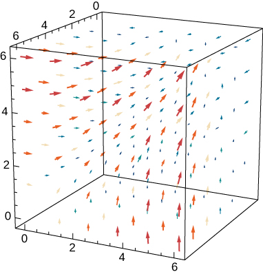
Figure 6.56 The curl of vector field
is zero.
The curl of F is
Thus, F is conservative.
We have seen that the curl of a gradient is zero. What is the divergence of a gradient? If
is a function of two variables, then
We abbreviate this “double dot product” as
This operator is called the Laplace operator, and in this notation Laplace’s equation becomes
Therefore, a harmonic function is a function that becomes zero after taking the divergence of a gradient.
Similarly, if
is a function of three variables then
Using this notation we get Laplace’s equation for harmonic functions of three variables:
Harmonic functions arise in many applications. For example, the potential function of an electrostatic field in a region of space that has no static charge is harmonic.
Example 6.57
Analyzing a Function
Is it possible for
to be the potential function of an electrostatic field that is located in a region of
free of static charge?
Solution
If
were such a potential function, then
would be harmonic. Note that
and
and so
Therefore,
is not harmonic and
cannot represent an electrostatic potential.
Checkpoint 6.46
Is it possible for function
to be the potential function of an electrostatic field located in a region of
free of static charge?
