
2. Vectors in Three Dimensions
Vectors are useful tools for solving two-dimensional problems. Life, however, happens in three dimensions. To expand the use of vectors to more realistic applications, it is necessary to create a framework for describing three-dimensional space. For example, although a two-dimensional map is a useful tool for navigating from one place to another, in some cases the topography of the land is important. Does your planned route go through the mountains? Do you have to cross a river? To appreciate fully the impact of these geographic features, you must use three dimensions. This section presents a natural extension of the two-dimensional Cartesian coordinate plane into three dimensions.
Three-Dimensional Coordinate Systems
As we have learned, the two-dimensional rectangular coordinate system contains two perpendicular axes: the horizontal x-axis and the vertical y-axis. We can add a third dimension, the z-axis, which is perpendicular to both the x-axis and the y-axis. We call this system the three-dimensional rectangular coordinate system. It represents the three dimensions we encounter in real life.
Definition
The three-dimensional rectangular coordinate system consists of three perpendicular axes: the x-axis, the y-axis, the z-axis, and an origin at the point of intersection (0) of the axes. Because each axis is a number line representing all real numbers in ℝ, the three-dimensional system is often denoted by ℝ3.
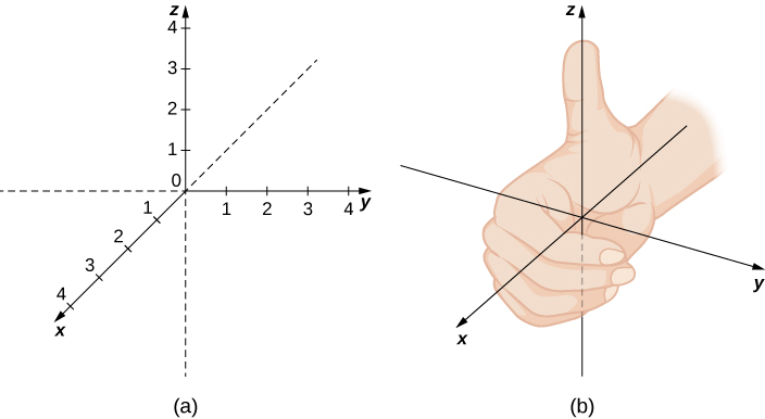
In Figure 3.2.1(a), the positive z-axis is shown above the plane containing the x– and y-axes. The positive x-axis appears to the left and the positive y-axis is to the right. A natural question to ask is: How was arrangement determined? The system displayed follows the right-hand rule. If we take our right hand and align the fingers with the positive x-axis, then curl the fingers so they point in the direction of the positive y-axis, our thumb points in the direction of the positive z-axis. In this text, we always work with coordinate systems set up in accordance with the right-hand rule. Some systems do follow a left-hand rule, but the right-hand rule is considered the standard representation.
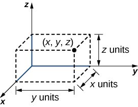
In two dimensions, we describe a point in the plane with the coordinates (x,y). Each coordinate describes how the point aligns with the corresponding axis. In three dimensions, a new coordinate, z, is appended to indicate alignment with the z-axis: (x,y,z). A point in space is identified by all three coordinates Figure 3.2.2. To plot the point (x,y,z), go x units along the x-axis, then y units in the direction of the y-axis, then z units in the direction of the z-axis.
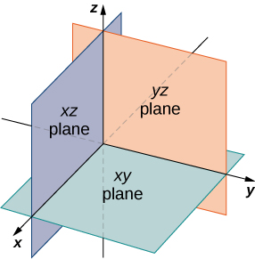
In two-dimensional space, the coordinate plane is defined by a pair of perpendicular axes. These axes allow us to name any location within the plane. In three dimensions, we define coordinate planes by the coordinate axes, just as in two dimensions. There are three axes now, so there are three intersecting pairs of axes. Each pair of axes forms a coordinate plane: the xy-plane, the xz-plane, and the yz-plane Figure 3.2.2. We define the xy-plane formally as the following set: { (x, y, 0) : x, y ∈ ℝ}. Similarly, the xz-plane and the yz-plane are defined as { (x, 0, z) : x, z ∈ ℝ}and { (0, y, z) : y, z ∈ ℝ}, respectively.
To visualize this, imagine you’re building a house and are standing in a room with only two of the four walls finished. (Assume the two finished walls are adjacent to each other.) If you stand with your back to the corner where the two finished walls meet, facing out into the room, the floor is the xy-plane, the wall to your right is the xz-plane, and the wall to your left is the yz-plane.
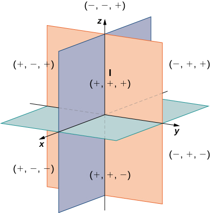
In two dimensions, the coordinate axes partition the plane into four quadrants. Similarly, the coordinate planes divide space between them into eight regions about the origin, called octants. The octants fill ℝ3 in the same way that quadrants fill ℝ2, as shown in Figure 3.2.4.
Most work in three-dimensional space is a comfortable extension of the corresponding concepts in two dimensions. In this section, we use our knowledge of circles to describe spheres, then we expand our understanding of vectors to three dimensions. To accomplish these goals, we begin by adapting the distance formula to three-dimensional space.
If two points lie in the same coordinate plane, then it is straightforward to calculate the distance between them. We that the distance d between two points (x1,y1) and (x2,y2) in the xy-coordinate plane is given by the formula

The formula for the distance between two points in space is a natural extension of this formula.
Theorem
The Distance between Two Points in Space
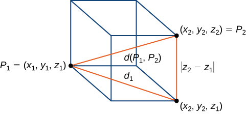
The distance d between points (x1,y1,z1) and (x2,y2,z2) is given by the formula

The proof of this theorem is left as an exercise. (Hint: First find the distance d1 between the points x1,y1,z1 and x2,y2,z1 as shown in Figure 3.2.5.)
Example: Distance in Space
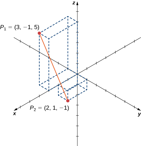
Find the distance between points P1=(3,−1,5) and P2=(2,1,−1).
Solution
Substitute values directly into the distance formula:

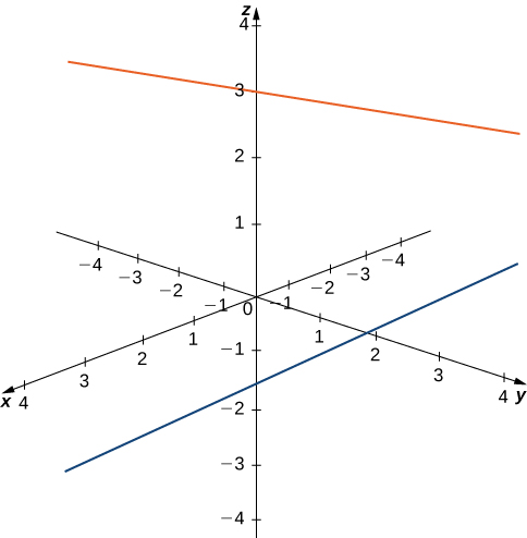
Before moving on to the next section, let’s get a feel for how ℝ3 differs from ℝ2. For example, in ℝ2, lines that are not parallel must always intersect. This is not the case in ℝ3.
For example, consider the line shown in Figure 3.2.6. These two lines are not parallel, nor do they intersect.
You can also have circles that are interconnected but have no points in common, as in Figure 3.2.7.
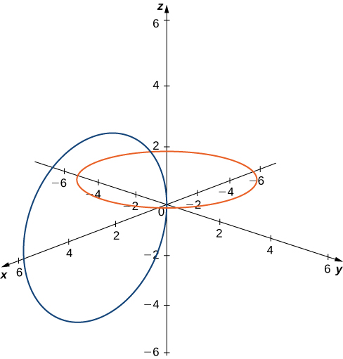
We have a lot more flexibility working in three dimensions than we do if we stuck with only two dimensions.
Writing Equations in ℝ3
Now that we can represent points in space and find the distance between them, we can learn how to write equations of geometric objects such as lines, planes, and curved surfaces in ℝ3. First, we start with a simple equation. Compare the graphs of the equation x=0 in ℝ, ℝ2, and ℝ3 (Figure 3.2.8). From these graphs, we can see the same equation can describe a point, a line, or a plane.
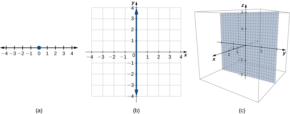
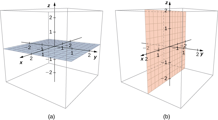
In space, the equation x=0 describes all points (0,y,z). This equation defines the yz-plane. Similarly, the xy-plane contains all points of the form (x,y,0). The equation z=0 defines the xy-plane and the equation y=0 describes the xz-plane (Figure 3.2.9).
Understanding the equations of the coordinate planes allows us to write an equation for any plane that is parallel to one of the coordinate planes. When a plane is parallel to the xy-plane, for example, the z-coordinate of each point in the plane has the same constant value. Only the x– and y-coordinates of points in that plane vary from point to point.
Rule: Equations of Planes Parallel to Coordinate Planes
- The plane in space that is parallel to the xy-plane and contains point (a,b,c) can be represented by the equation z=c.
- The plane in space that is parallel to the xz-plane and contains point (a,b,c)can be represented by the equation y=b.
- The plane in space that is parallel to the yz-plane and contains point (a,b,c)can be represented by the equation x=a.
As we have seen, in ℝ2 the equation x=5 describes the vertical line passing through point (5,0). This line is parallel to the y-axis. In a natural extension, the equation x=5 in ℝ3 describes the plane passing through point (5,0,0), which is parallel to the yz-plane. Another natural extension of a familiar equation is found in the equation of a sphere.
Definition
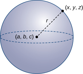
A sphere is the set of all points in space equidistant from a fixed point, the center of the sphere, just as the set of all points in a plane that are equidistant from the center represents a circle. In a sphere, as in a circle, the distance from the center to a point on the sphere is called the radius.
The equation of a circle is derived using the distance formula in two dimensions. In the same way, the equation of a sphere is based on the three-dimensional formula for distance.
Rule: Equation of a Sphere
The sphere with center a,b,c and radius r can be represented by the equation

Working with Vectors in ℝ3
Just like two-dimensional vectors, three-dimensional vectors are quantities with both magnitude and direction, and they are represented by directed line segments (arrows). With a three-dimensional vector, we use a three-dimensional arrow.
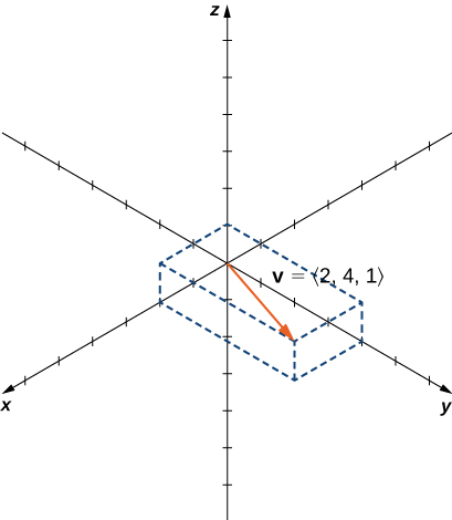
Three-dimensional vectors can also be represented in component form. The notation v= is a natural extension of the two-dimensional case, representing a vector with the initial point at the origin, (0,0,0), and terminal point (x,y,z). The zero vector is 0=
 . So, for example, the three dimensional vector v=
 is represented by a directed line segment from point (0,0,0) to point (2,4,1) (Figure 3.2.10).
Vector addition and scalar multiplication are defined analogously to the two-dimensional case. If v= and w=
 are vectors, and k is a scalar, then
v+w=  and kv =
If k=-1, then kv=-1v is written as –v, and vector subtraction is defined by v–w=v+-w=v+-1w.
The standard unit vectors extend easily into three dimensions as well — i= , j=
, j= , and k=
 — and we use them in the same way we used the standard unit vectors in two dimensions. Thus, we can represent a vector in ℝ3 in the following ways:
v =  = xi +yj +zk
Example: Vector Representations
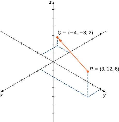
Let  be the vector with initial point P=(3,12,6) and terminal point Q=(-4,-3,2) as shown below. Express in both component form and using standard unit vectors.
Solution
In component form,

In standard unit form,
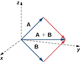
=-7i-15j-4k.As described earlier, vectors in three dimensions behave in the same way as vectors in a plane. The geometric interpretation of vector addition, for example, is the same in both two- and three-dimensional space (Figure 3.2.11).
We have already seen how some of the algebraic properties of vectors, such as vector addition and scalar multiplication, can be extended to three dimensions. Other properties can be extended in similar fashion. They are summarized here for our reference.
Rule: Properties of Vectors in Space
Let v= and w= be vectors, and let k be a scalar.
Scalar multiplication: kv=
Vector addition: v+w= + = 
Vector subtraction: v–w= –  =
= 
Vector magnitude: v= 
We have seen that vector addition in two dimensions satisfies the commutative, associative, and additive inverse properties. These properties of vector operations are valid for three-dimensional vectors as well. Scalar multiplication of vectors satisfies the distributive property, and the zero vector acts as an additive identity. The proofs to verify these properties in three dimensions are straightforward extensions of the proofs in two dimensions.
