In this section, we examine two important operations on a vector field: divergence and curl. They are important to the field of calculus for several reasons, including the use of curl and divergence to develop some higher-dimensional versions of the Fundamental Theorem of Calculus. In addition, curl and divergence appear in mathematical descriptions of fluid mechanics, electromagnetism, and elasticity theory, which are important concepts in physics and engineering. We can also apply curl and divergence to other concepts we already explored. For example, under certain conditions, a vector field is conservative if and only if its curl is zero.

In addition to defining curl and divergence, we look at some physical interpretations of them, and show their relationship to conservative and source-free vector fields.

Divergence

Divergence is an operation on a vector field that tells us how the field behaves toward or away from a point. Locally, the divergence of a vector field F in ℝ² or ℝ³ at a particular point P is a measure of the “outflowing-ness” of the vector field at P. If F represents the velocity of a fluid, then the divergence of F at P measures the net rate of change with respect to time of the amount of fluid flowing away from P (the tendency of the fluid to flow “out of” P). In particular, if the amount of fluid flowing into P is the same as the amount flowing out, then the divergence at P is zero.

Definition

Note the divergence of a vector field is not a vector field, but a scalar function. In terms of the gradient operator ∇ = 〈 〉 divergence can be written symbolically as the dot product

Note this is merely helpful notation, because the dot product of a vector of operators and a vector of functions is not meaningfully defined given our current definition of dot product.

If F=〈P, Q〉 is a vector field in ℝ², and P_x and Q_y both exist, then the divergence of F is defined similarly as

div F = = = ∇⋅F.

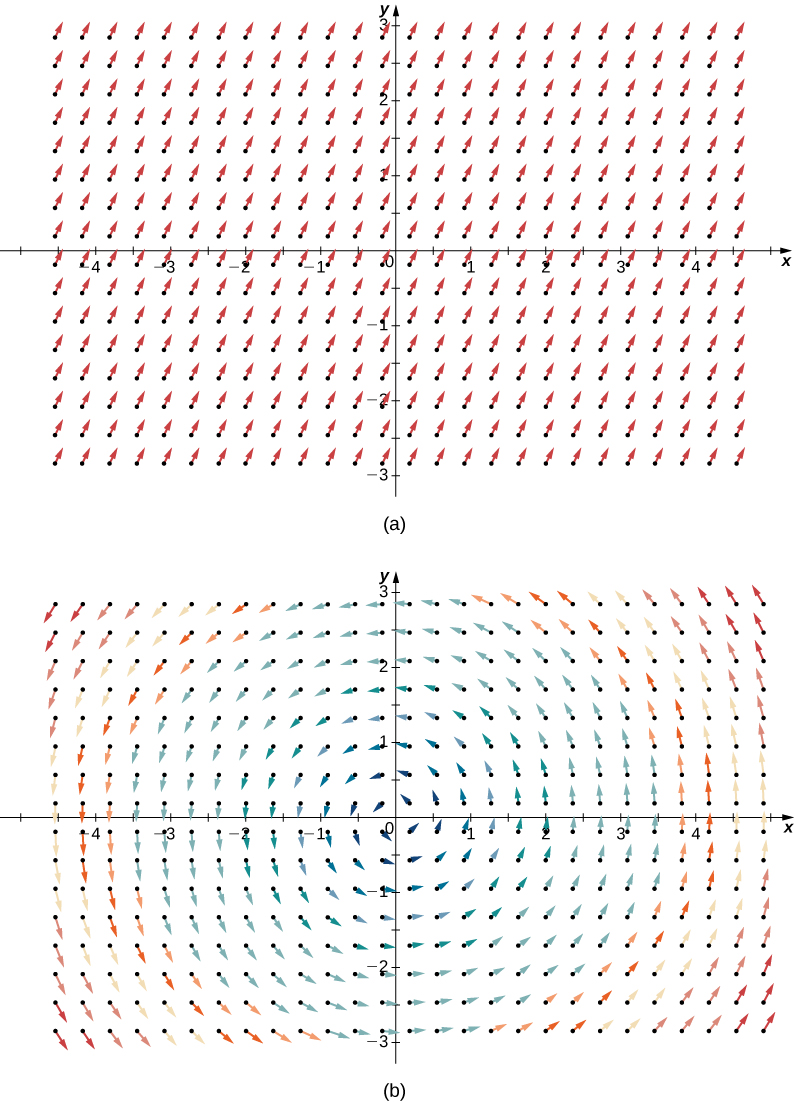
To illustrate this point, consider the two vector fields in Figure 3.7.1. At any particular point, the amount flowing in is the same as the amount flowing out, so at every point the “outflowing-ness” of the field is zero. Therefore, we expect the divergence of both fields to be zero, and this is indeed the case, as

By contrast, consider radial vector field R(x,y)=〈−x,−y〉 in Figure 3.7.2. At any given point, more fluid is flowing in than is flowing out, and therefore the “outgoingness” of the field is negative. We expect the divergence of this field to be negative, and this is indeed the case, as div(R) = = -2.

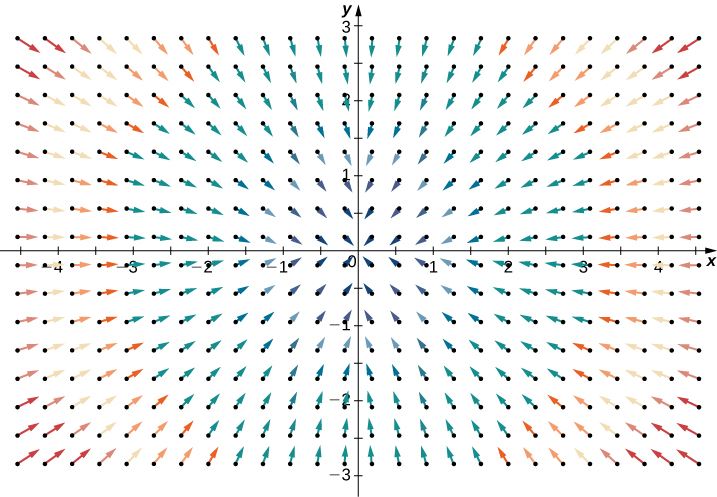
To get a global sense of what divergence is telling us, suppose that a vector field in ℝ²  represents the velocity of a fluid. Imagine taking an elastic circle (a circle with a shape that can be changed by the vector field) and dropping it into a fluid. If the circle maintains its exact area as it flows through the fluid, then the divergence is zero. This would occur for both vector fields in Figure 3.7.1. On the other hand, if the circle’s shape is distorted so that its area shrinks or expands, then the divergence is not zero. Imagine dropping such an elastic circle into the radial vector field in Figure 3.7.2 so that the center of the circle lands at point (3, 3). The circle would flow toward the origin, and as it did so the front of the circle would travel more slowly than the back, causing the circle to “scrunch” and lose area. This is how you can see a negative divergence.

One application for divergence is detecting whether a field is source free. Recall that a source-free field is a vector field that has a stream function; equivalently, a source-free field is a field with a flux that is zero along any closed curve. The next two theorems say that, under certain conditions, source-free vector fields are precisely the vector fields with zero divergence.

Theorem

Proof

Since F is source free, there is a function g(x,y)with g_y=P and −g_x=Q. Therefore, F=〈g_y,−g_x〉 and div F=〈g_yx−g_xy〉 = 0 by Clairaut’s theorem.

□

The converse of Divergence of a Source-Free Vector Field is true on simply connected regions, but the proof is too technical to include here. Thus, we have the following theorem, which can test whether a vector field in ℝ² is source free.

Theorem

Recall that the flux form of Green’s theorem says that

=

where C is a simple closed curve and D is the region enclosed by C. Since P_x+Q_y=div F, Green’s theorem is sometimes written as

=

Therefore, Green’s theorem can be written in terms of divergence. If we think of divergence as a derivative of sorts, then Green’s theorem says the “derivative” of F on a region can be translated into a line integral of F along the boundary of the region. This is analogous to the Fundamental Theorem of Calculus, in which the derivative of a function f on a line segment [a,b] can be translated into a statement about f on the boundary of [a,b]. Using divergence, we can see that Green’s theorem is a higher-dimensional analog of the Fundamental Theorem of Calculus.

We can use all of what we have learned in the application of divergence. Let v be a vector field modeling the velocity of a fluid. Since the divergence of v at point P measures the “outflowing-ness” of the fluid at P, div v(P)>0 implies that more fluid is flowing out of P than flowing in. Similarly, div v(P)<0 implies the more fluid is flowing in to P  than is flowing out, and div v(P)=0 implies the same amount of fluid is flowing in as flowing out.

Curl

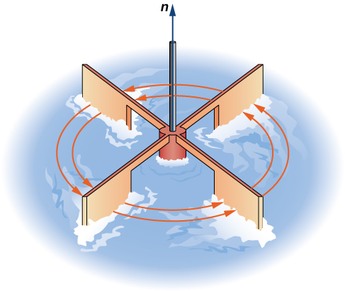
The second operation on a vector field that we examine is the curl, which measures the extent of rotation of the field about a point. Suppose that F represents the velocity field of a fluid. Then, the curl of F at point P is a vector that measures the tendency of particles near P to rotate about the axis that points in the direction of this vector. The magnitude of the curl vector at P measures how quickly the particles rotate around this axis. In other words, the curl at a point is a measure of the vector field’s “spin” at that point. Visually, imagine placing a paddlewheel into a fluid at P, with the axis of the paddlewheel aligned with the curl vector (Figure 3.7.3). The curl measures the tendency of the paddlewheel to rotate.

Consider the vector fields in Figure 3.7.1. In part (a), the vector field is constant and there is no spin at any point. Therefore, we expect the curl of the field to be zero, and this is indeed the case. Part (b) shows a rotational field, so the field has spin. In particular, if you place a paddlewheel into a field at any point so that the axis of the wheel is perpendicular to a plane, the wheel rotates counterclockwise. Therefore, we expect the curl of the field to be nonzero, and this is indeed the case (the curl is 2k).

To see what curl is measuring globally, imagine dropping a leaf into the fluid. As the leaf moves along with the fluid flow, the curl measures the tendency of the leaf to rotate. If the curl is zero, then the leaf doesn’t rotate as it moves through the fluid.

Definition

The definition of curl can be difficult to remember. To help with remembering, we use the notation ∇ × F to stand for a “determinant” that gives the curl formula:

The determinant of this matrix is

Thus, this matrix is a way to help remember the formula for curl. Keep in mind, though, that the word determinant is used very loosely. A determinant is not really defined on a matrix with entries that are three vectors, three operators, and three functions.

If F = 〈P,Q〉 is a vector field in ℝ², then the curl of F, by definition, is

Note that if F=〈P,Q〉 is a vector field in a plane, then curl F⋅k=(Q_x−P_y)k⋅k=Q_x−P_y. Therefore, the circulation form of Green’s theorem is sometimes written as

=,

where C is a simple closed curve and D is the region enclosed by C. Therefore, the circulation form of Green’s theorem can be written in terms of the curl. If we think of curl as a derivative of sorts, then Green’s theorem says that the “derivative” of F on a region can be translated into a line integral of F along the boundary of the region. This is analogous to the Fundamental Theorem of Calculus, in which the derivative of a function f on line segment [a,b] can be translated into a statement about f on the boundary of [a,b]. Using curl, we can see the circulation form of Green’s theorem is a higher-dimensional analog of the Fundamental Theorem of Calculus.

Using Divergence and Curl

Now that we understand the basic concepts of divergence and curl, we can discuss their properties and establish relationships between them and conservative vector fields.

If F is a vector field in ℝ³, then the curl of F is also a vector field in ℝ³. Therefore, we can take the divergence of a curl. The next theorem says that the result is always zero. This result is useful because it gives us a way to show that some vector fields are not the curl of any other field. To give this result a physical interpretation, recall that divergence of a velocity field v at point P measures the tendency of the corresponding fluid to flow out of P. Since div curl v=0, the net rate of flow in vector field curl(v) at any point is zero. Taking the curl of vector field F eliminates whatever divergence was present in F.

Theorem

Proof

By the definitions of divergence and curl, and by Clairaut’s theorem,

□

With the next two theorems, we show that if F is a conservative vector field then its curl is zero, and if the domain of F is simply connected then the converse is also true. This gives us another way to test whether a vector field is conservative.

Theorem

Proof

Since conservative vector fields satisfy the cross-partials property, all the cross-partials of F are equal. Therefore,

□

The same theorem is true for vector fields in a plane.

Since a conservative vector field is the gradient of a scalar function, the previous theorem says that curl (∇f)=0 for any scalar function f. In terms of our curl notation, ∇ × (∇f)=0. This equation makes sense because the cross product of a vector with itself is always the zero vector. Sometimes equation ∇ × ∇(f)=0 is simplified as ∇ × ∇=0.

Theorem

Proof

Since curl F=0, we have that R_y=Q_z, P_z=R_x, and Q_x=P_y. Therefore, F satisfies the cross-partials property on a simply connected domain, and Cross-Partial Property of Conservative Fields implies that F is conservative.

□

The same theorem is also true in a plane. Therefore, if F is a vector field in a plane or in space and the domain is simply connected, then F is conservative if and only if

We have seen that the curl of a gradient is zero. What is the divergence of a gradient? If f is a function of two variables, then div(∇f)=∇⋅(∇f)=f_xx+f_yy. We abbreviate this “double dot product” as ∇². This operator is called the Laplace operator, and in this notation Laplace’s equation becomes ∇²f=0. Therefore, a harmonic function is a function that becomes zero after taking the divergence of a gradient.

Similarly, if f is a function of three variables then

Using this notation we get Laplace’s equation for harmonic functions of three variables: