In this section, we develop an operation called the dot product, which allows us to calculate work in the case when the force vector and the motion vector have different directions. The dot product essentially tells us how much of the force vector is applied in the direction of the motion vector. The dot product can also help us measure the angle formed by a pair of vectors and the position of a vector relative to the coordinate axes. It even provides a simple test to determine whether two vectors meet at a right angle.

The Dot Product and Its Properties

We have already learned how to add and subtract vectors. In this chapter, we investigate two types of vector multiplication. The first type of vector multiplication is called the dot product, based on the notation we use for it, and it is defined as follows:

Definition

The dot product of vectors u= and v= is given by the sum of the products of the components

u⋅v = .

Note that if u and v are two-dimensional vectors, we calculate the dot product in a similar fashion. Thus, if  u= and v=, then:

u⋅v =

When two vectors are combined under addition or subtraction, the result is a vector. When two vectors are combined using the dot product, the result is a scalar. For this reason, the dot product is often called the scalar product. It may also be called the inner product.

Like vector addition and subtraction, the dot product has several algebraic properties. We prove three of these properties and leave the rest as exercises.

Theorem 2.3

Proof

Let  u= and v=. Then

The associative property looks like the associative property for real-number multiplication, but pay close attention to the difference between scalar and vector objects:

The proof that c (u⋅v) = u ⋅ (c v) is similar.

The fourth property shows the relationship between the magnitude of a vector and its dot product with itself:

□

Note that the definition of the dot product yields 0⋅v=0. By property iv., if v⋅v=0, then v=0.

Using the Dot Product to Find the Angle between Two Vectors

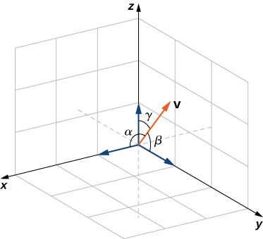
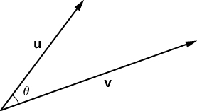
When two nonzero vectors are placed in standard position, whether in two dimensions or three dimensions, they form an angle between them (Figure 3.3.1). The dot product provides a way to find the measure of this angle. This property is a result of the fact that we can express the dot product in terms of the cosine of the angle formed by two vectors.

Theorem

Proof

Place vectors u and v in standard position and consider the vector v–u (Figure 3.3.2). These three vectors form a triangle with side lengths ||u||, ||v||, and ||v−u||.

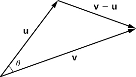
Recall from trigonometry that the law of cosines describes the relationship among the side lengths of the triangle and the angle θ. Applying the law of cosines here gives

The dot product provides a way to rewrite the left side of this equation:

Substituting into the law of cosines yields

□

We can use this form of the dot product to find the measure of the angle between two nonzero vectors. The following equation rearranges the equation above to solve for the cosine of the angle:

cos θ=.

Using this equation, we can find the cosine of the angle between two nonzero vectors. Since we are considering the smallest angle between the vectors, we assume 0°≤θ≤180° (or 0≤θ≤π if we are working in radians). The inverse cosine is unique over this range, so we are then able to determine the measure of the angle θ.

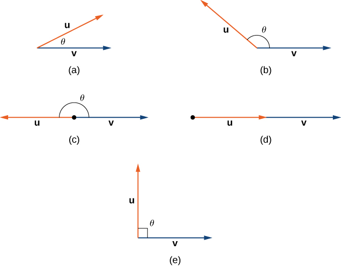
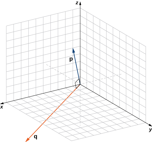
The angle between two vectors can be acute (0<cos θ<1), obtuse (−1<cos θ<0), or straight (cos θ=−1.) If cos θ=1, then both vectors have the same direction. If cos θ=0, then the vectors, when placed in standard position, form a right angle (Figure 3.3.3). We can formalize this result into a theorem regarding orthogonal (perpendicular) vectors.

Theorem

Proof

Let u and v be nonzero vectors, and let θ denote the angle between them. First, assume u⋅v=0. Then

However, ||u||≠0 and ||v||≠0, so we must have cos θ=0. Hence, θ=90°, and the vectors are orthogonal. Now assume u and v are orthogonal. Then θ=90° and we have

□

The terms orthogonal, perpendicular, and normal each indicate that mathematical objects are intersecting at right angles. The use of each term is determined mainly by its context. We say that vectors are orthogonal and lines are perpendicular. The term normal is used most often when measuring the angle made with a plane or other surface.

Example: Identifying Orthogonal Vectors

Determine whether p= and q= are orthogonal vectors.

Solution

Using the definition, we need only check the dot product of the vectors:

p⋅q=1(10)+(0)(3)+(5)(−2)=10+0−10=0.

Because p⋅q=0, the vectors are orthogonal.

The angle a vector makes with each of the coordinate axes, called a direction angle, is very important in practical computations, especially in a field such as engineering. For example, in astronautical engineering, the angle at which a rocket is launched must be determined very precisely. A very small error in the angle can lead to the rocket going hundreds of miles off course. Direction angles are often calculated by using the dot product and the cosines of the angles, called the direction cosines. Therefore, we define both these angles and their cosines.

Definition