
4. Drag and Inertia Coefficients
In the previous section, we established that Morison’s equation, an empirically derived formula, allows us to predict loads on narrow bodies in oscillatory flow (such as waves). The inline force,  , due to a combination of drag and inertia, is expressed by:

In this equation:
 is the fluid density (kg/m3)
 and
and  are dimensionless coefficients representing drag and inertia, respectively,
 is the projected area normal to the flow,
- U is the fluid velocity, and
 is the volume of the body.
The central question becomes: what values should we assign to the coefficients and ? These coefficients play a critical role in accurately predicting the force on the body.
Drag Coefficient
The drag coefficient, , quantifies the resistive force due to the flow around a body and is dimensionless. It is defined by the relation:

where:
-
 is the force (N) in the direction of the flow,
- U is the fluid velocity (m/s), and
- A is the frontal projected area of the body (m2).
You can verify that is indeed dimensionless by checking the units in this equation. This formula is particularly useful when the drag force is already known. However, when predicting the drag force, we need to select an appropriate value of based on the body’s characteristics and its interaction with the flow.
Selecting a Drag Coefficient Based on Shape and Reynolds Number
The choice of depends heavily on the shape of the object and the flow conditions, often characterized by the Reynolds number (Re), which incorporates flow velocity, object diameter, and fluid viscosity. Researchers have extensively measured and simulated drag forces across various shapes and flow rates, leading to drag coefficient charts that plot against Re. There is ample published research on experimentally and numerically (computer simulation) determined values for the drag coefficients of cylinders and a wide range of airfoils. Work on other shapes is sparser, but still available for shapes such as squares.
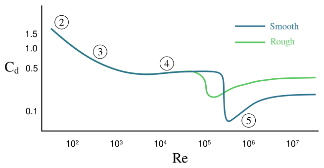
For example, Figure 9.4.1 shows a graph of for a sphere in uniform flow across different Reynolds numbers. This chart distinguishes between a smooth and a rough sphere surface and indicates distinct flow regimes that impact the drag coefficient:
- Region 2: Attached flow (Stokes flow) and steady separated flow,
- Region 3: Separated unsteady flow with a laminar boundary layer, producing a vortex street,
- Region 4: Unsteady flow with a laminar boundary layer before separation, and a turbulent wake downstream,
- Region 5: Super-critical flow with a turbulent boundary layer before separation.
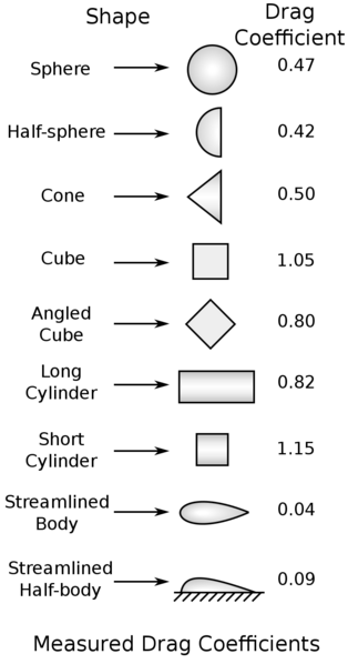
Extensive empirical data also exists for cylinders and airfoils, with limited data for square or non-standard shapes. Figure 9.4.2 provides a reference for drag coefficients of various geometries, though it applies specifically to cases with a Reynolds number of 10.
Inertia Coefficient
The inertia coefficient, , accounts for the additional force from accelerating fluid around the body. Similar to is often derived from experimental or high-fidelity simulation data and varies according to the body’s shape and flow characteristics.
Typically, is presented graphically with the Keulegan-Carpenter (KC) number on the horizontal axis, where KC compares the relative importance of drag to inertia forces. Charts of as a function of KC can be found in academic literature, providing guidance based on specific geometries.
Unlike drag coefficients, which often remain below unity (one), inertia coefficients can exceed a value of two, reflecting the significant contribution of inertia forces in some flow scenarios. These coefficients are crucial for modeling oscillatory flows accurately and are selected based on the body’s geometry and flow conditions.
Summary
Morison’s equation provides a framework for predicting loads on narrow bodies in oscillatory flows by incorporating drag and inertia effects. The choice of the coefficients and is key to accurate predictions and requires careful consideration of the body’s shape, Reynolds number, and the nature of the flow.
