2. Modeling Irregular Waves

Maija Benitz

2. Modeling Irregular Waves

In this chapter, we shift from the regular, fully predictable waves discussed in the previous section to the complex, irregular waves that define much of the ocean surface. Unlike regular waves, which are repetitive and characterized by a single frequency and amplitude, irregular waves feature a range of wave heights and frequencies, as shown in Figure 8.2.1. To model these irregular, stochastic waves, we must use probabilistic methods and spectral analysis, as a single wave description cannot capture their variability.

**Figure 8.2.1** Image of a rogue wave in the western North Atlantic during the Atlantic Remote Sensing Land/Ocean Experiment (ARSLOE) that depicts the sea surface comprised of many wave heights and frequencies. (Image by Bronson Fotiadis [CC BY 4.0], via Wikimedia Commons).

**Figure 8.2.2** A regular wave that has one height and one frequency. (Photo by digicla [CC BY 2.0], via Wikimedia Commons).

Wave Superposition

We saw in the previous section that waves interact with each to create interference patterns that can be constructive, destructive, or mixed. The mixed interference pattern shown in Figure 8.1.4 showed a wave that was the result of a combination of constructive and destructive interference, producing a new wave train that contained multiple heights and frequencies. In fact, the mixed interference led to a wave train that looked irregular, or more like the sea surface.

To create these mixed interference patterns we need to begin with individual wave trains that can be summed together. These individual wave contributions can be represented with any of the wave theories we discussed in the previous chapter, including Airy waves, Stokes 1st Order, 2nd Order, cnoidal, etc. The choice of theory depends on the region of applicability, also discussed in the previous chapter.

Suppose that our environmental conditions under consideration land us in the linear theory (Airy waves) region of Figure 7.6.7. A regular linear wave — that is, one that is comprised of a single wave amplitude and frequency — is represented as a function of time by the equation below.

$\eta = A \cos(\omega t + \phi)$

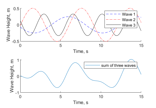
where A is the wave amplitude, $\omega$ is the wave frequency, t is time, and $\phi$ is a random phase angle. For sake of example, let’s consider three waves each with their own heights, frequencies, and phase shifts, as represented in the top plot of Figure 8.2.3.

We can model the irregular waves at our site by summing together multiple linear wave components (or terms), each with their own height and frequency compositions. The wave height, $\eta$ , for an irregular wave as a function of time is therefore represented as,

$\eta = A_1 \cos(\omega_1 t + \phi_1) + A_2 \cos(\omega_2 t + \phi_2) ...+ A_N \cos(\omega_N t + \phi_N)$

where the subscripts on each variable indicate the individual wave contribution, allowing for up to N number of terms. In our example, we are summing three terms, so N = 3. The result of combining the three regular waves is shown in the bottom plot of Figure 8.2.3 by a wave that appears to contain multiple heights and frequencies.

**Figure 8.2.3** (Top) Three regular waves with different heights, frequencies, and phase shifts are shown, (Bottom) the result of summing the three wave trains is shown.

A few questions should arise in your mind at this point. Namely,

What values should be used for wave amptlitude, A, and frequency, $\omega$ , so that we are creating waves that represent the ocean?
How do we ensure that our summation of waves are physically representative of our ocean environment? That is, how many terms, N, are appropriate or even necessary?

Wave Spectra

Our ability to model engineering applications in the ocean environment relies on accurately predicting the responses of structures in realistic random seas. Therefore, we need a way to describe the sea surface accurately and appropriately, which is not easy, as we have already recognized that ocean waves contain many wave heights and periods. One approach to characterizing the surface is to use a spectrum, that is a mathematical description of the distribution of wave energy as a function of wave frequency. Though many formulations have been developed since the 1950s, here we’ll explore the two mostly commonly used spectra (or spectrums); the Pierson-Moskowitz and the Joint North Sea Wave Observation Project (JONSWAP). Both of the spectra discussed here rely on measurements from the ocean.

Spectral analysis can feel very complex or intangible. For this text, it suffices to think of a spectrum as a description of the ocean waves that are the result of wind blowing over a long distance for several days. It is almost like a biography of the waves at a location — a depiction of their size and temporal nature.

Pierson-Moskowitz

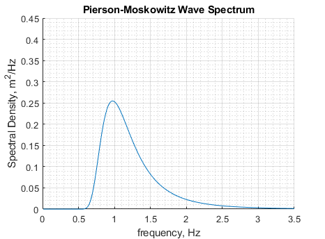
The Pierson-Moskowitz spectrum is named for the two scientists who proposed it in 1964, based on measurements collected in the North Atlantic. This spectrum assumes fully developed seas, that assumes waves are in equilibrium with the wind which has blown steadily over a long distance and time period. The general spectral formulation, S, is given as a function of wave frequency, $\omega$ , as follows,

$S(\omega) = \frac{A g^2}{\omega^5} exp[-B (\frac{\omega}{\omega_0})^4]$

where $A = 8.1 * 10^{-3}$ , $B = 0.74$ , $\omega_0 = g/U_{19.5}$ , and $U_{19.5}$ is the wind speed measured 19.5 m above the sea surface. The $exp$ terms means exponential, as in $e^x$ . Note that the Pierson-Moskowitz Spectrum is a function of one variable — the wave frequency, $\omega$ . The spectrum is shown visually in Figure 8.2.4 below, using ocean conditions measured by a National Oceanic and Atmospheric Administration (NOAA) weather buoy in Port Orford, OR in 2016.

**Figure 8.2.4** A representation of the Pierson-Moskowitz spectrum, based on sea conditions at Port Orford, OR in 2016.

JONSWAP

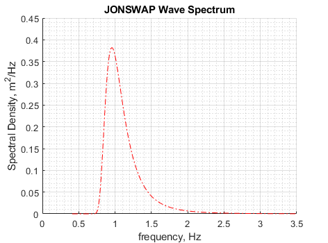
Just over a decade later, a new measurement campaign was undertaken in the North Sea in 1968 and 1969 call the Joint North Sea Wave Observation Project (JONSWAP). In contrast to the Pierson-Moskowitz spectrum, this work found that the waves were never fully-developed, thus providing a new spectrum for fetch limited seas. Perhaps unsurprisingly, the mathematical formulation of the JONSWAP spectrum is very similar to that of Pierson-Moskowitz, in that is primarily comprised of an exponential term that is a function of wave frequency. A peak enhancement term is added to the Pierson-Moskowitz spectrum, which accounts for fetch and results in a sharper peak. The JONSWAP spectrum gives S as a function of wave frequency, $\omega$ , as follows,

$S(\omega) = \frac{A g^2}{\omega^5} exp[-\frac{5}{4} (\frac{\omega_p}{\omega})^4] \gamma^r$

The differences between the two spectra are worth noting in more detail. Firstly, in the JONSWAP equation, $A = 0.076 (\frac{U_{10}}{Fg})^{0.22}$ , where $U_{10}$ is the wind speed at 10 meters above the sea surface and F is the fetch (distance over which the wind has blown). This is especially notable, as the Pierson-Moskowitz spectrum does not include any consideration of fetch, as it assumes a fully developed sea. Further, $\omega_p$ representing the peak wave frequency, is given by $0.877g/U_{19.5}$ . Finally, the last term, given by $\gamma^r$ , is called the peak enhancement factor. The value of $\gamma$ falls between 1 and 6, and is often given by 3.3. Its exponent r is given by $r = exp[\frac{-(\omega-\omega_p)}{2 \sigma^2 \omega_p^2}]$ , where $\sigma$ equals 0.07 when $\omega \leq \omega_p$ and 0.09 otherwise.

The JONSWAP spectrum is shown in Figure 8.2.5 below.

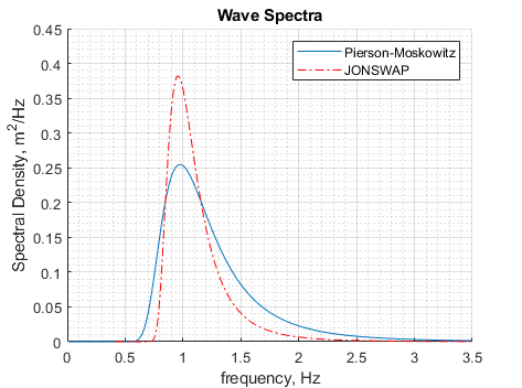
**Figure 8.2.5** A representation of the JONSWAP spectrum.

A comparison of the two spectra is shown in Figure 8.2.6 below, illustrating the narrower peak of the JONSWAP.

**Figure 8.2.6** Comparison of the Pierson-Moskowitz (blue line) and JONSWAP (red dash-dot) spectra.

Modeling Random Seas

We are now ready to answer the questions that were posed earlier in this section:

What values should be used for wave amplitude, A, and frequency, $\omega$ , so that we are creating waves that represent the ocean?
How do we ensure that our summation of waves are physically representative of our ocean environment? That is, how many terms, N, are appropriate or even necessary?

Our first goal is to determine values for the wave amplitude, A, and frequency, $\omega$ , that are representative of our ocean environment. We don’t want to randomly draw these values out of a hat or dream them up off the tops of our heads — that would lead to waves that are completely arbitrary and not necessarily representative of wave characteristics at our site. So, to answer the first question, let’s consider the Pierson-Moskowitz spectrum given in Figure 8.2.7.

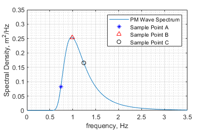
**Figure 8.2.7** Three sample points on the Pierson-Moskowitz Spectrum for Port Orford, OR in 2016. These points will determine the wave heights and frequencies for representative waves in a superposition.

For sake of simplicity, three sample points A, B, and C are shown on the Pierson-Moskowitz spectrum, with a blue star, red triangle, and black circle, respectively. We are searching for amplitudes in units of meters and frequencies in units of Hertz. Conveniently those units appear on the x- and y-axes of our spectrum. The frequency is more direct, as all we need to do it take the x-value of each sample point to determine the wave frequency that wave component.

Next, we recognize that the product of the units on the x- and y-axes gives $\frac{m^2}{Hz} * Hz = m^2$ . So to determine an amplitude in meters, we can take the square root of that product, $\sqrt{ \frac{m^2}{Hz} * Hz} = \sqrt{m^2} = m$ . Thus, the wave amplitude for a sample point, $n$ , is given by $A_n = \sqrt{S_n * \omega_n}$ , where $S_n$ is the spectral density value found on the y-axis and $\omega_n$ is the corresponding frequency on the x-axis. Recall that some randomness is introduced via the random phase angle, $\phi$ , such that each wave is shifted differently in the side-side direction.

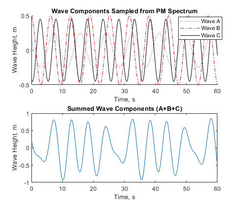
**Figure 8.2.8** (Top) Three waves created by sampling the Pierson-Moskowitz spectrum at points A, B, and C (Bottom) The result of summing the three wave components as a function of time.

The waves produced with the amplitudes and frequencies determined at each of the three sample points are shown in top plot of Figure 8.2.8. The sum of the three waves is shown in the bottom plot of Figure 8.2.8 exhibiting multiple wave heights and frequencies, though a pattern of repetition is still quite apparent. And so we arrive at the crux of our second question — how many waves do we need to sum to produce an irregular wave that accurately represents the sea surface?

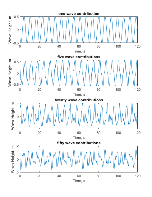
The answer is best demonstrated visually. Consider the plots shown in Figure 8.2.9, where one, five, twenty, and fifty waves are summed together, in the top, middle two, and bottom plots, respectively. As more wave heights and frequencies are included, via summing more terms, the resulting waves become increasingly irregular. That is, any underlying repetition becomes harder to detect, as the waves as many heights, frequencies, and phase angles as the number of contributing terms in the summation. Since our goal is to create irregular waves, we recognize that more terms is better. But just how many? In practice, somewhere in the neighborhood of 50 terms is sufficient.

**Figure 8.2.9** The superposition of differing number of components, from one at the top, to five, twenty, and finally fifty terms at the bottom. The superpositions with higher number of contributions display more randomness, which is our goal.

License

Icon for the Creative Commons Attribution-NonCommercial-ShareAlike 4.0 International License