Many different processes play important roles in the climate system.  Here we discuss atmospheric and oceanic circulations, how they transport heat and water, and we’ll explore a little more in depth Earth’s water cycle and how it penetrates all climate system components and is linked to the energy cycle.

Atmospheric Circulation

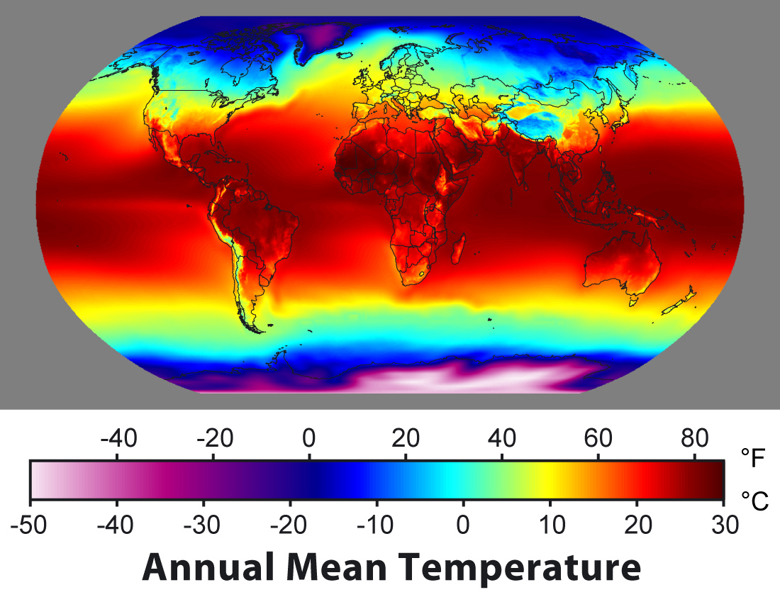
Annual mean surface temperatures on Earth range from less than −40°C in Antarctica to +30°C in the tropics (Figure 1.4.1). This begs the question: why is it warmer in the tropics than at the poles? The answer is, of course, because there is more sunlight in the tropics.

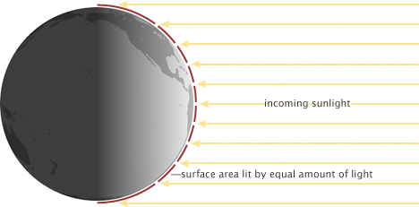
Due to the curvature of Earth’s surface the equator receives more incident solar radiation per area than the poles (Figure 1.4.2). Most solar radiation is received on a surface perpendicular to the sun’s rays, whereas the more tilted Earth’s surface is with respect to the sun’s rays the less energy it receives. This is similar to holding a flashlight perpendicular to a surface or at an angle. The area lit is smaller if the flashlight shines perpendicular onto the surface. This configuration maximizes the energy input. The area lit is larger the larger the angle between the flashlight and the surface. In the extreme case of a 90° angle, or more, there is no light at all received. This situation corresponds to the poles or the dark side of the Earth.

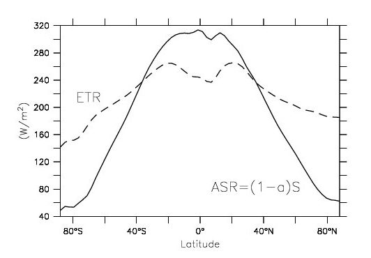
Satellites have measured radiative fluxes at the top-of-the-atmosphere. Those data can be used to calculate the heat gain from absorbed solar radiation (ASR) and the heat loss from emitted terrestrial radiation (ETR) as a function of latitude (Figure 1.4.3). The data show ASR values of around 300 Wm^-2 in the tropics and 60 Wm^-2 at the poles. Thus, the equator-to-pole difference is about 240 Wm^-2. However, values for the ETR are only around 250 Wm^-2 in the tropics and between 150 and 200 Wm^-2 at the poles. Thus, the equator-to-pole difference is only about 50 to 100 Wm^-2. The difference between the absorbed and emitted radiation gives the net heat gain from these fluxes. In the tropics the gain is positive. That is, there is more energy gain than energy loss. At the poles, on the other hand, there is more energy loss than energy gain. Therefore, if no other processes were involved the equator would warm up and the poles would cool down. But this is not the case, which implies a heat transport from the tropics towards the poles.

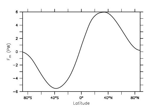
Taking the difference ASR – ETR and integrating it from one pole to the other gives the total meridional heat flux (Figure 1.4.4). In the southern hemisphere values are negative indicating southward heat transport. Positive values in the northern hemisphere represent northward transport. Poleward heat fluxes are peak at mid-latitudes with values of between 5 and 6 PW.

Most of the meridional heat transport is carried by the atmosphere (4-5 PW) whereas the ocean is responsible for a smaller portion (1-2 PW). Complex and turbulent motions in the atmosphere such as seen in visualizations from satellites play an important part in this heat transfer.

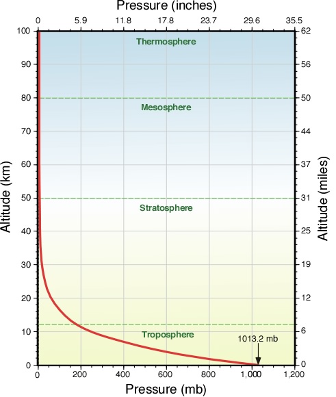
Air is compressible. The weight of overlaying air compresses the air beneath and increases the pressure closer to the surface (Figure 1.4.5). Therefore, pressure decreases with height and the surface pressure depends on the density and mass of the air above.

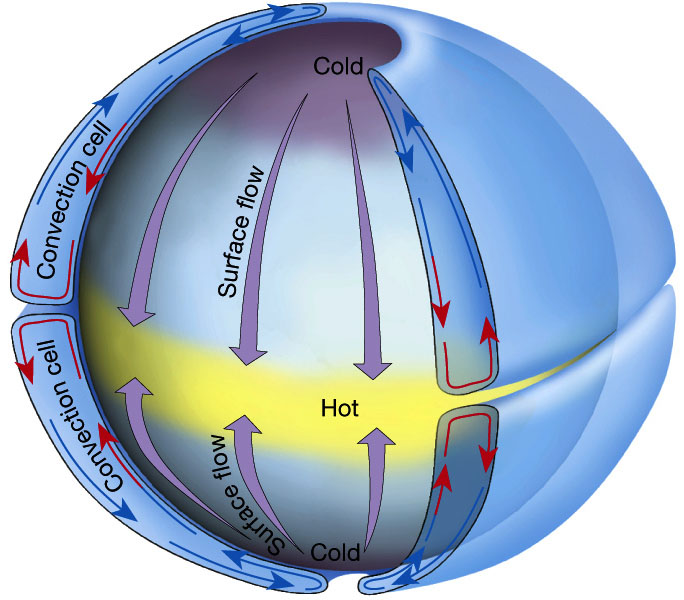
Let’s imagine a non-rotating Earth (Figure 1.4.6). In this case, the air at the poles would be cold and the air at the equator would be hot. Since colder air is denser than warm air the pressure at the north pole would be larger than at the equator. The air at the equator would rise and the air at the poles would sink. At the surface, the air would flow from high to low pressure, thus from the poles to the equator. At high altitudes the air would move from the equator to the poles.

However, Earth does rotate, which creates the Coriolis effect. Earth’s rotation causes a deflection of air and water masses towards the right (left) in the northern (southern) hemisphere. The Coriolis force is a consequence of angular momentum conservation. Assume an air parcel at rest at the equator. (An analogy would be a spinning ice dancer with extended arms.) Its angular momentum is M = R×U, where U = 40,000 km/day = 500 m/s is approximately the velocity of the Earth at the equator. Now move the air northward. (The ice dancer pulls his/her arms in.) This will decrease R. In order to conserve angular momentum U has to increase. If the air moved to about 60°N its distance from the axis of rotation would have decreased by about one half. Therefore, U must have doubled. Thus, the air parcel would have a velocity of 500 m/s relative to the Earth’s surface. Such high speeds never occur on Earth because of friction and turbulence but this simple example still explains qualitatively the high eastward wind velocities of around 40 m/s observed in the mid-latitude jet streams (Figure 1.4.7).

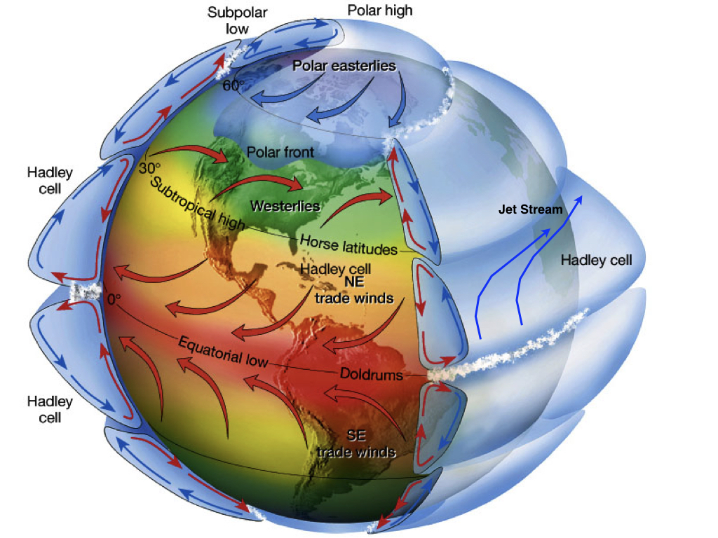
Rising of warm moist air at the equator causes water vapor condensation due to cooling of the air during the ascent. Clouds form and precipitation occurs. Some of the deepest cumulonimbus clouds on Earth form in the tropics.  They can reach the top of the troposphere or higher. The cool relatively dry air then moves poleward. Now the Coriolis effect kicks in, deflects the air towards the right (left) in the northern (southern) hemisphere, which creates the jet stream. The air cools by emitting longwave radiation to space. This increases the density and the air descends back to the surface in the subtropics (~30°N/S). During the descend the air warms and its relative humidity decreases. This leads to dry conditions in the subtropics indicated by the major deserts at those latitudes.

Subsequently the dry air moves back towards the equator. The Coriolis force deflects it towards the right (left) in the northern (southern) hemisphere, creating the easterly trade winds in the tropics. During this movement along the sea surface the air picks up water vapor from evaporation. Once the air returns to the equator it is saturated with water vapor (close to 100% relative humidity). The resulting meridional overturning cells in the tropical atmosphere are called Hadley cells, or Hadley circulation. Two cells, one in each hemisphere, exist only during the fall and spring, whereas during summer/winter there is only one major cell with rising air just slightly off the equator in the summer hemisphere, where the heating is largest.

The belt of rising air close to the equator is called the Intertropical Convergence Zone (ITCZ), due to the convergence of air along the surface. The ITCZ is further north in the northern hemisphere summer and further south in the southern hemisphere summer, although on average it is slightly north of the equator because the northern hemisphere is slightly warmer than the southern hemisphere due to ocean heat transport from the southern to the northern hemisphere (Frierson et al., 2013).

Surface air moving from the high pressure at subtropical latitudes towards lower pressure at mid-latitudes also experiences the Coriolis effect. This leads to the prevailing westerly winds at mid-latitudes. Another important feature of the atmospheric circulation at mid-latitudes is the growth, movement, and decay of synoptic weather systems (transient eddies) that dominate weather variability and heat transport there. Transient eddies are the low and high pressure systems that move eastward, some of which can be associated with storms.

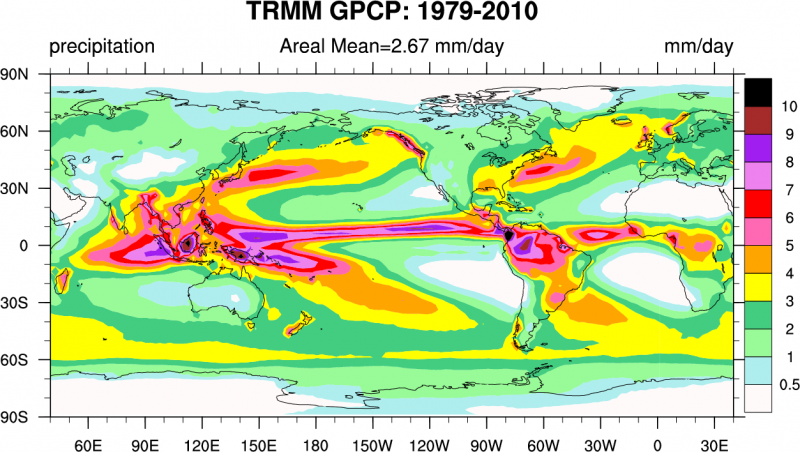
Explore these features of the global atmospheric circulation in this animation of weather variations throughout a whole year from satellite observations. You may notice the pulsing of convection over tropical Africa and South America. This is caused by the diurnal (daily) cycle of surface heating. Figure (1.4.8) shows the observed global distribution of precipitation. Note the ITCZ as the band of high precipitation close to the equator, the regions of low precipitation in the subtropics and the bands of high precipitation at mid-latitudes in the paths of the storm tracks over the North Pacific and North Atlantic. In the southern hemisphere we see an additional band between 50-60°S.

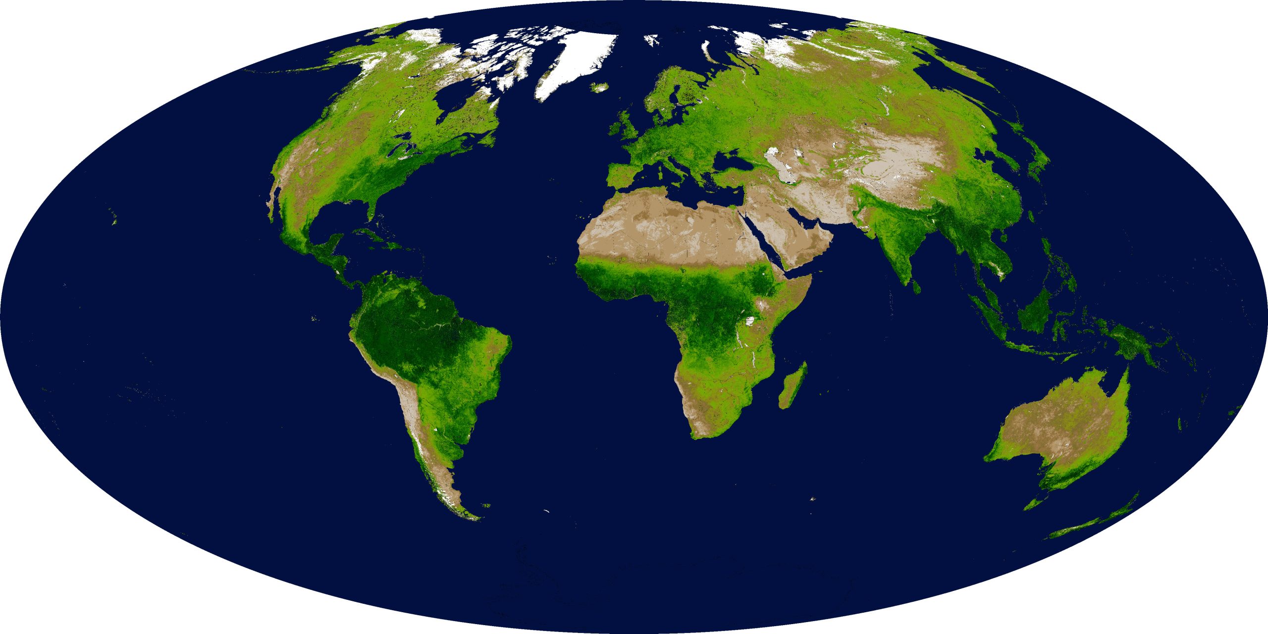
Precipitation has a strong effect on vegetation as can be seen from the similarities between Figures 1.4.8 and 1.4.9. Regions of large precipitation such as tropical Africa, South America, and Asia have dense vegetation, whereas regions of little precipitation such as the Sahara, the Arabian Peninsula, regions in central Asia, southwestern parts of North America, central and western Australia, parts of South America west of the Andes, and southwestern Africa also have sparse desert or steppe vegetation. This relation is not a surprise considering that photosynthesis requires water.

Ocean Circulation

The general, planetary-scale circulation of the ocean can be separated into a wind-driven component that dominates the upper ocean and a density driven component that occupies the deep ocean. Five large gyres are the main features of the surface circulation in the subtropics (Figure 1.4.10). The easterly trade winds push water towards the west in the tropics. The water piles up where it encounters land and flows poleward. The poleward flow brings warm waters from the tropics to the mid-latitudes. There, the westerly winds push the surface waters toward the east. Again, where the current hits a continent it piles up and flows north and south. The southward flowing part completes the subtropical gyre bringing cold waters towards the tropics. The poleward flow along the western boundaries of the subtropical gyres are warm currents, such as the Gulf Stream, the Kuroshio, and the Brazil Currents. Equatorward currents along the eastern boundaries are cold such as the California or the Peru (or Humboldt) Currents. Within the subtropical gyres the water flows in a spiral-like pattern towards the center of the gyre. This convergence causes sinking in the centers of the gyres. However, the water is relatively warm so it sinks only to depths of a few hundred meters. In the tropics, on the other hand, the trade winds cause divergence and upwelling.

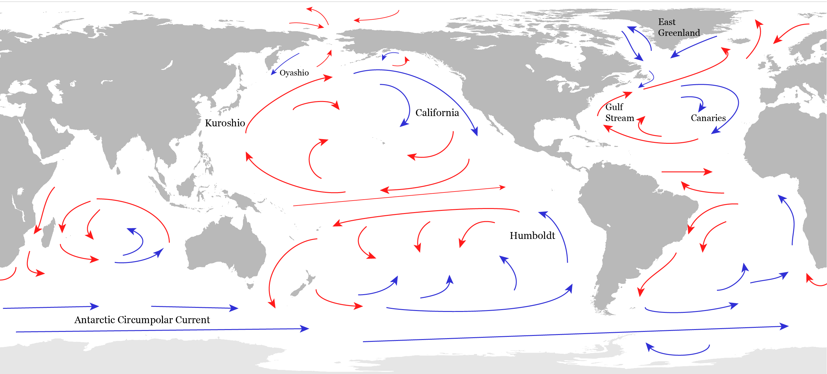
Surface currents near the equator are particularly vigorous. The piling up of waters in the western equatorial Pacific, for example, causes the narrow Equatorial Counter Current to move eastward.

The strongest current in the world oceans is the Antarctic Circumpolar Current, which transports more than 100 million cubic meters of water per second around Antarctica flowing eastward. That amounts to 500 times the Amazon river discharge. The Southern Ocean is also an important region for upwelling of deep waters caused by a wind-driven divergence of surface waters.

Watch a high resolution model simulation of surface ocean currents here. It shows more details such as mesoscale eddies, which are the ocean’s equivalent of weather systems in the atmosphere. Notice that they are much smaller in size than high and low pressure systems in the atmosphere due to the larger density of seawater compared with air. Try to identify some of the features discussed above such as the Gulf Stream and the Antarctic Circumpolar Current. These and other fascinating features are also seen in satellite observations of sea surface temperatures here and here.

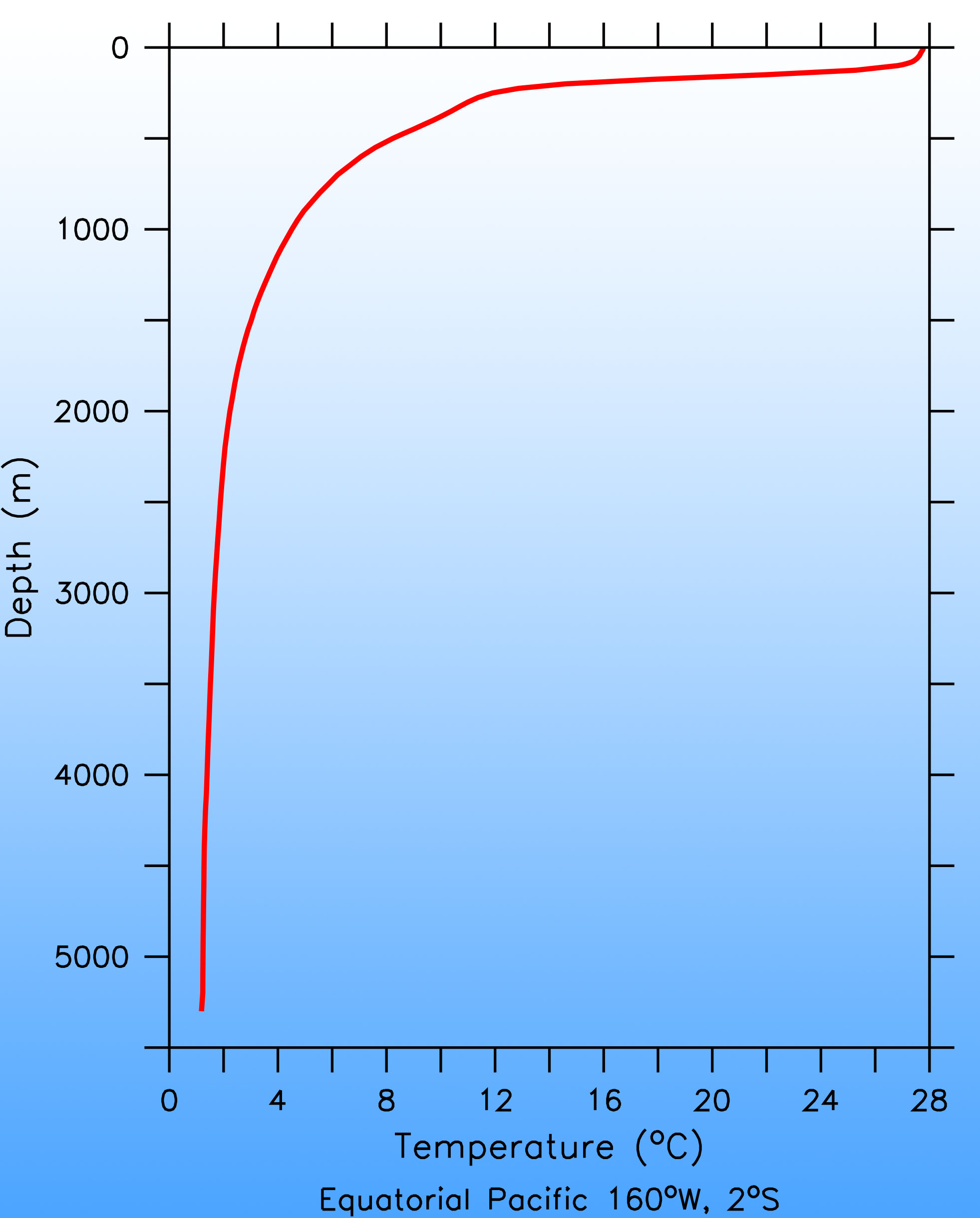
In contrast to the atmosphere, the ocean is mostly stably stratified. That is, denser water is layered below lighter water. The density of sea water is determined by temperature and salinity. The colder and saltier, the heavier it is. Typically warmer, more buoyant water is on top of colder water, especially at low latitudes (Figure 1.4.11). This is because water absorbs sunlight efficiently, which heats the surface. Winds cause lots of turbulence close to the surface, which creates a layer of uniform temperature called the surface mixed layer. Below that, between about 200 – 1000 m depth, is a region in which the temperature decreases rapidly with depth. This is called the thermocline. Turbulence is weak here. Further down is the weakly stratified deep and abyssal ocean. Vertical temperature gradients are small here. Closer to the sea floor turbulence increases due to interactions of flow with the bottom topography.

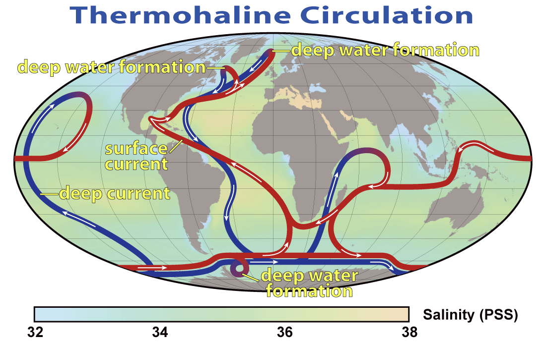
The deep ocean is cold because waters there originate from the high-latitude surface. Only in a few regions of the world’s oceans where the density of surface waters is large enough do they sink into the deep ocean (Figure 1.4.12). In the current ocean there is deep water formation in the North Atlantic and near Antarctica. Surface waters of the Atlantic are saltier than those of the Pacific because of water vapor transport within the atmosphere. Whereas mountain ranges at mid-latitudes block water vapor transport from the Pacific to the Atlantic with the westerly winds there, in the tropics gaps in the mountains allow water vapor transport with the trade winds from the Atlantic to the Pacific. This causes fresher, more buoyant surface waters in the Pacific. In the North Pacific this freshwater lens prevents sinking, whereas in the North Atlantic saltier waters are dense enough to sink to about 2-3 km depth. From there they flow south along the margin of the Americas pushed there by the Coriolis force. The deep water from the North Atlantic crosses the equator and the South Atlantic and enters into the Southern Ocean. Part of it rises back to the surface there whereas the rest flows into the Indian and Pacific Oceans, where it slowly ascends. The return flow at the surface flows through the Indonesian Archipelago into the Indian Ocean, merges with upwelled waters there and continues to flow westward around the tip of South Africa and back northward across the Atlantic. This planetary scale circulation pattern is called the thermohaline (thermo = temperature, haline = salinity) circulation or meridional (north-south) overturning circulation.

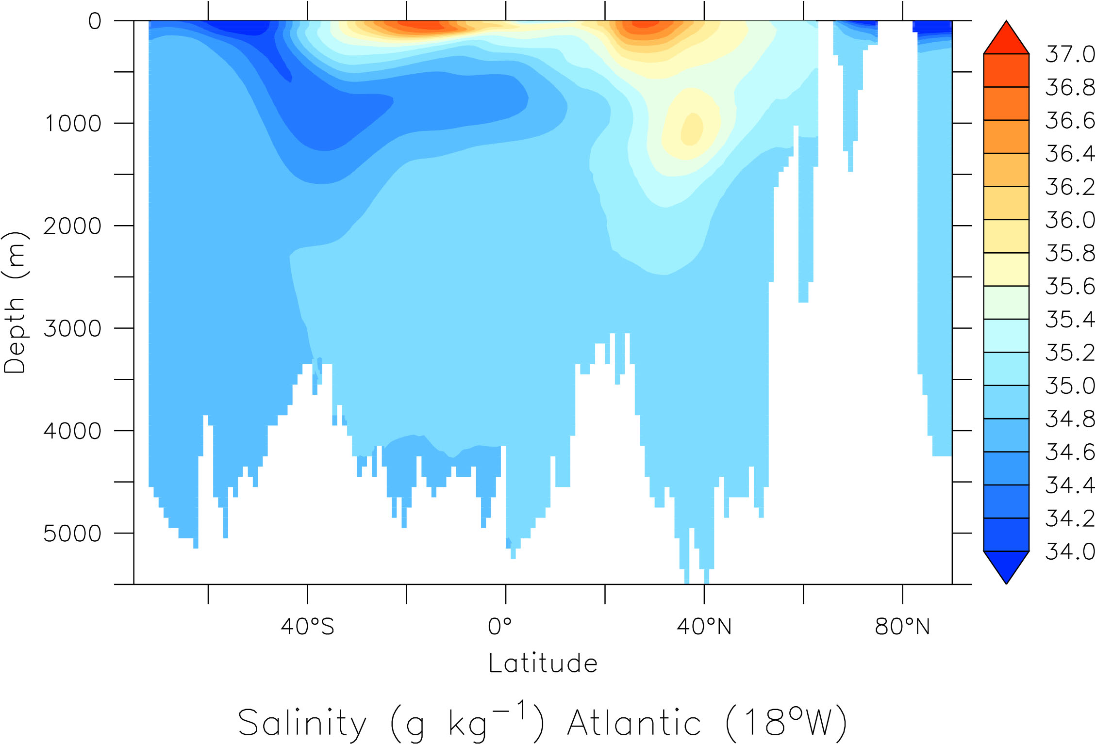
Its circulation impacts tracer distributions in the ocean (Figure 1.4.13). E.g. in the Atlantic the southward flowing North Atlantic Deep Water (NADW) can be identified as a water mass with relatively high salinity between about 2 – 4 km depth. Fresher Antarctic Bottom Water (AABW) flows north below NADW. It is colder and therefore denser than NADW. Relatively fresh Antarctic Intermediate Water (AAIW) flows north above NADW creating a sandwich-like structure in the deep Atlantic. In the North Atlantic there is a blob of high salinity water around 1 km depth and 40°N. This is outflow from the Mediterranean Sea, which is very salty.

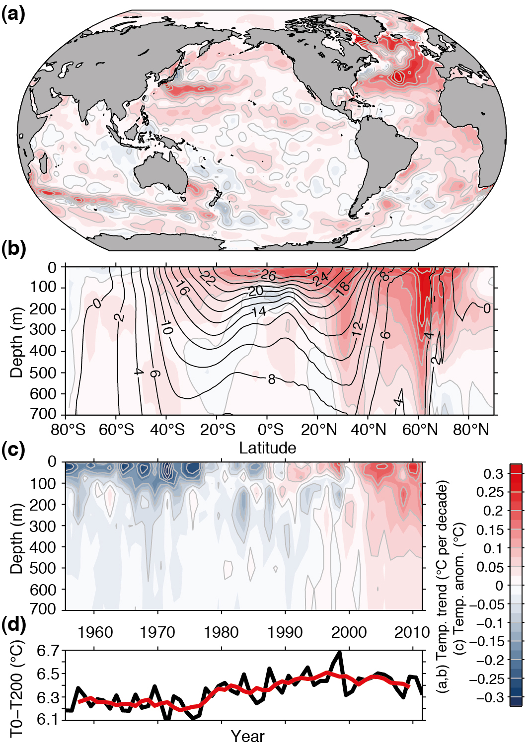
Observations show that the ocean is warming (Figure 1.4.14). Most of the increase in temperatures is concentrated near the surface consistent with a warming atmosphere as its cause. A prominent maximum of heat uptake is in the North Atlantic, similar to the pattern of anthropogenic carbon uptake. The reason is the sinking and southward penetration of NADW, which transports both anthropogenic carbon and heat from the surface to the deep ocean there. Other regions of enhanced heat uptake are the subtropics, where surface waters sink to a few hundred meters depth in the centers of the subtropical gyres. Ocean temperature observations rule out that changes in ocean circulation are the cause of the observed warming of the surface. If this was the case deeper layers would have cooled, which is not what is observed. Therefore, the hypothesis that changes in ocean circulation have caused the observed warming of the atmosphere during the past 50 years has been falsified by subsurface temperature observations.

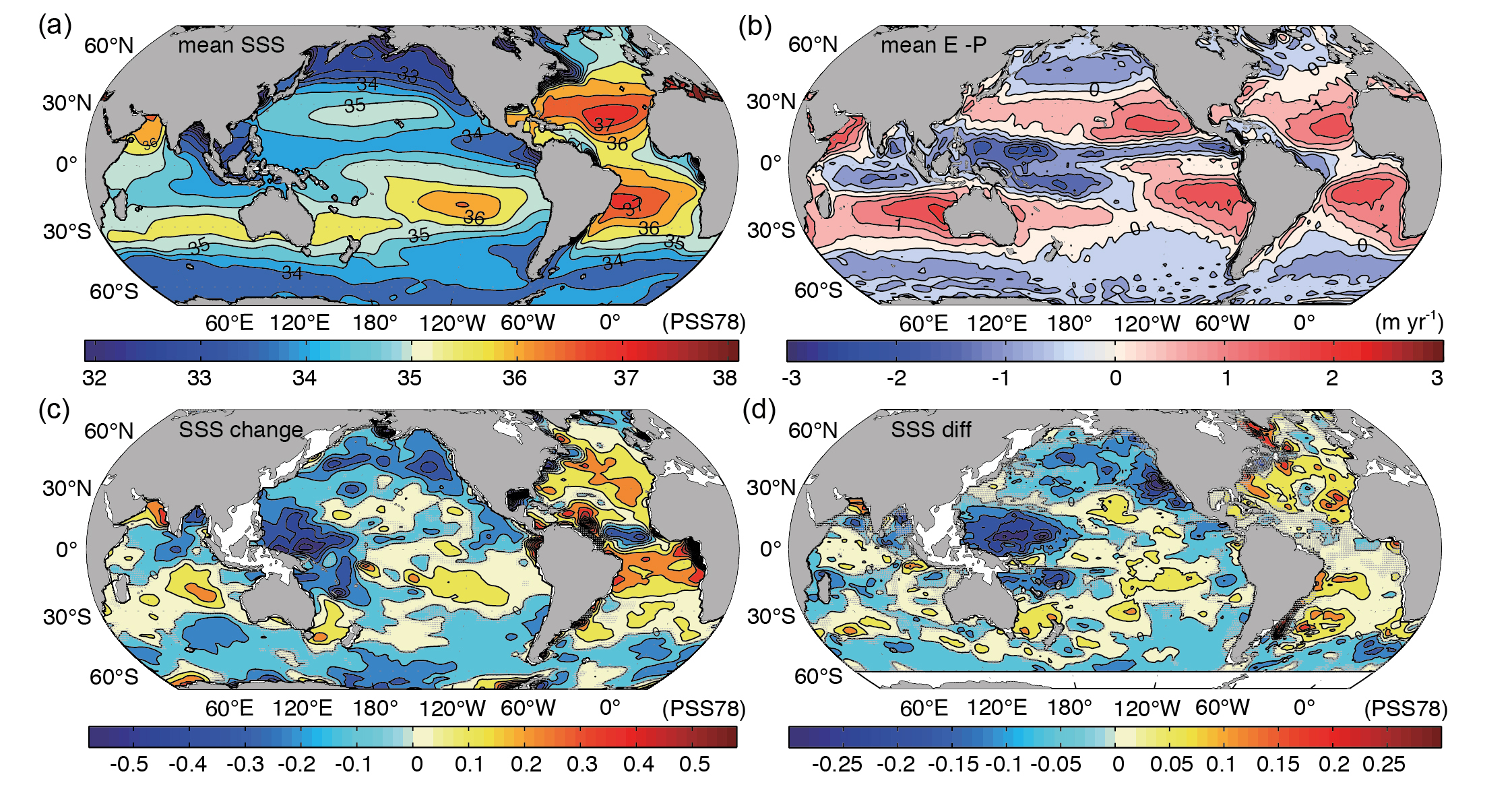
Acceleration of the atmospheric hydrological cycle also affects ocean surface salinities (Figure 1.4.15). Regions that are already salty such as the subtropics and the Atlantic get even saltier and regions that are already fresh like the North Pacific and the Southern Ocean get even fresher.

Warming and freshening of surface waters at high latitudes decreases their density and increases their buoyancy. This reduces deep water formation and the meridional overturning circulation. A reduction of the Atlantic meridional overturning circulation, which was initially predicted by climate models in the 1990’s (Manabe and Stouffer, 1993), is now observed in measurements from the subtropical Atlantic (Smeed et al., 2014). However, due to the relatively short period of the available data (2004 to the present) it is currently not clear how much of the observed reduction is caused by human greenhouse gas emissions and how much is due to natural variability. A long-term decline of the Atlantic meridional overturning circulation has been suggested by Rahmstorf et al. (2015) to cause the reduced warming over the subpolar North Atlantic in surface temperature observations (Section 2, Figure 1.2.2). Here is a nice interactive article about the topic.

Videos

YouTube: How Ocean Circulation Works from It’s Okay To Be Smart

References

Frierson, D. M. W., Y.-T. Hwang, N. S. Fuckar, R. Seager, S. M. Kang, A. Donohoe, E. A. Maroon, X. Liu, and D. S. Battisti (2013), Contribution of ocean overturning circulation to tropical rainfall peak in the Northern Hemisphere, Nature Geosci, 6(11), 940-944, doi:10.1038/ngeo1987.

Hartmann, D.L., A.M.G. Klein Tank, M. Rusticucci, L.V. Alexander, S. Brönnimann, Y. Charabi, F.J. Dentener, E.J. Dlugokencky, D.R. Easterling, A. Kaplan, B.J. Soden, P.W. Thorne, M. Wild and P.M. Zhai, 2013: Observations: Atmosphere and Surface. In: Climate Change 2013: The Physical Science Basis. Contribution of Working Group I to the Fifth Assessment Report of the Intergovernmental Panel on Climate Change [Stocker, T.F., D. Qin, G.-K. Plattner, M. Tignor, S.K. Allen, J. Boschung, A. Nauels, Y. Xia, V. Bex and P.M. Midgley (eds.)]. Cambridge University Press, Cambridge, United Kingdom and New York, NY, USA.

Manabe, S., and R. J. Stouffer (1993), Century-Scale Effects of Increased Atmospheric CO2 on the Ocean-Atmosphere System, Nature, 364(6434), 215-218, doi: 10.1038/364215a0.

Peixoto, J., and A. Oort (1992) Physics of Climate, AIP Press.

Rahmstorf, S., J. E. Box, G. Feulner, M. E. Mann, A. Robinson, S. Rutherford, and E. J. Schaffernicht (2015), Exceptional twentieth-century slowdown in Atlantic Ocean overturning circulation, Nature Climate Change, 5(5), 475-480, doi: 10.1038/Nclimate2554.

Rhein, M., S.R. Rintoul, S. Aoki, E. Campos, D. Chambers, R.A. Feely, S. Gulev, G.C. Johnson, S.A. Josey, A. Kostianoy, C. Mauritzen, D. Roemmich, L.D. Talley and F. Wang, 2013: Observations: Ocean. In: Climate Change 2013: The Physical Science Basis. Contribution of Working Group I to the Fifth Assessment Report of the Intergovernmental Panel on Climate Change [Stocker, T.F., D. Qin, G.-K. Plattner, M. Tignor, S.K. Allen, J. Boschung, A. Nauels, Y. Xia, V. Bex and P.M. Midgley (eds.)]. Cambridge University Press, Cambridge, United Kingdom and New York, NY, USA.

Smeed, D. A., G. D. McCarthy, S. A. Cunningham, E. Frajka-Williams, D. Rayner, W. E. Johns, C. S. Meinen, M. O. Baringer, B. I. Moat, A. Duchez, and H. L. Bryden (2014), Observed decline of the Atlantic meridional overturning circulation 2004-2012, Ocean Sci., 10(1), 29-38, doi: 10.5194/os-10-29-2014.

Trenberth, K. E., L. Smith, T. Qian, A. Dai, and J. Fasullo (2007), Estimates of the Global Water Budget and Its Annual Cycle Using Observational and Model Data, Journal of Hydrometeorology, 8(4), 758-769, doi:10.1175/jhm600.1.