
5.3 Salinity Patterns
All of the salts and ions that dissolve in seawater contribute to its overall salinity. Salinity of seawater is usually expressed as the grams of salt per kilogram (1000 g) of seawater. On average, about 35 g of salt is present in each 1 kg of seawater, so we say that the average salinity of the ocean salinity is 35 parts per thousand (ppt). Note that 35 ppt is equivalent to 3.5% (parts per hundred). Some sources now use practical salinity units (PSU) to express salinity values, where 1 PSU = 1 ppt. The units are not included, so we can refer simply to a salinity of 35.
Many different substances are dissolved in the ocean, but six ions comprise about 99.4% of all the dissolved ions in seawater. These six major ions are (Table 5.3.1):
Table 5.3.1 The six major ions in seawater
| g/kg in seawater | % of ions by weight | |
|---|---|---|
| Chloride Cl- | 19.35 | 55.07% |
| Sodium Na+ | 10.76 | 30.6% |
| Sulfate SO42- | 2.71 | 7.72% |
| Magnesium Mg2+ | 1.29 | 3.68% |
| Calcium Ca2+ | 0.41 | 1.17% |
| Potassium K+ | 0.39 | 1.1% |
| 99.36% |
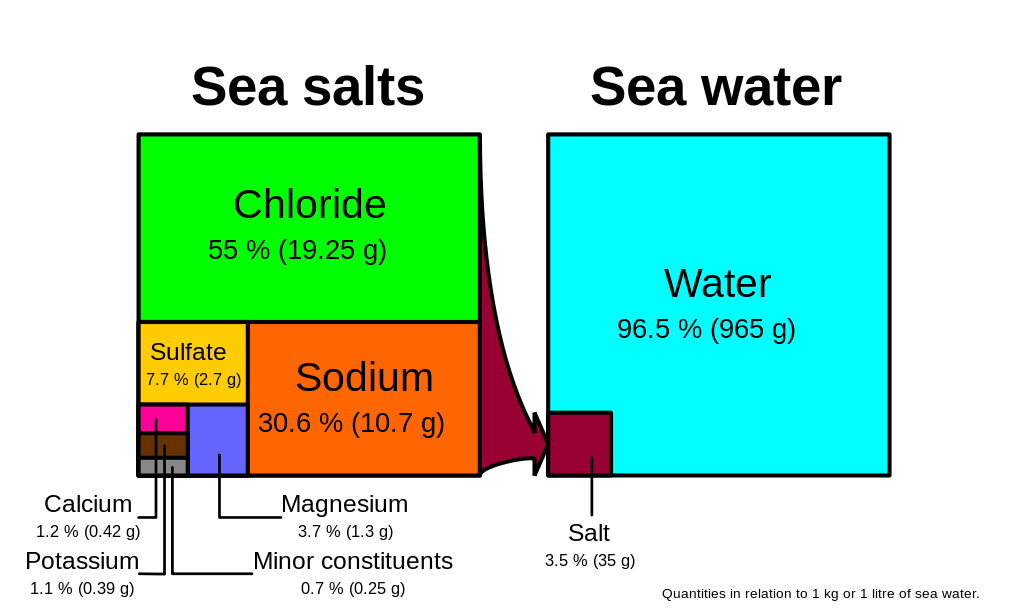
Chloride and sodium, the components of table salt (sodium chloride NaCl), make up over 85% of the ions in the ocean, which is why seawater tastes salty (Figure 5.3.1). In addition to the major constituents, there are numerous minor constituents; radionucleotides, organic compounds, metals etc. These minor constituents are found in concentrations of ppm (parts per million) or ppb (parts per billion), unlike the major ions that are far more abundant (ppt) (Table 5.3.2). To put this into perspective, 1 ppm = 1 mg/kg, or the equivalent of 1 teaspoon of sugar dissolved in 14,000 cans of soda. 1 ppb = 1 μg/kg, or the equivalent of 1 teaspoon of a substance dissolved in five Olympic-sized swimming pools! These minor constituents represent numerous substances, but together they make up less than 1% of the ions in the seawater. Some of these may be important as minerals and trace elements vital to living organisms, but they don’t have much impact on the overall salinity. But given the vast size of the oceans, even materials found in trace abundance can represent fairly large reservoirs. For example gold is a trace element in seawater, found in concentrations of parts per trillion, yet if you could extract all of the gold in just one km3 of seawater, it would be worth about $20 million!
Table 5.3.2 Concentrations of some minor elements in seawater
| g/kg in seawater | g/kg in seawater | ||
|---|---|---|---|
| Carbon | 0.028 | Iron | 2 x 10⁻⁶ |
| Nitrogen | 0.0115 | Manganese | 2 x 10⁻⁷ |
| Oxygen | 0.006 | Copper | 1 x 10⁻⁷ |
| Silicon | 0.002 | Mercury | 3 x 10⁻⁸ |
| Phosphorous | 6 x 10⁻⁵ | Gold | 4 x 10⁻⁹ |
| Uranium | 3.2 x 10⁻⁶ | Lead | 5 x 10⁻¹⁰ |
| Aluminum | 2 x 10⁻⁶ | Radon | 6 x 10-19 |
Because the six major ions in seawater comprise over 99% of the total salinity, changes in abundance of the minor constituents have little effect on overall salinity. Furthermore, the rule of constant proportions states that even though the absolute salinity of ocean water might differ in different places, the relative proportions of the six major ions within that water are always constant. For example, no matter the total salinity of a seawater sample, 55% of the total salinity will be due to chloride, 30% due to sodium, and so on. Since the proportion of these major ions does not change, we call these conservative ions.
Given these constant proportions, in order to calculate total salinity you can simply measure the concentration of just one of the major ions and use that value to calculate the rest. Traditionally chloride has been the ion measured because it is the most abundant, and thus the simplest to measure accurately. Multiplying the concentration of chloride by 1.8 gives the total salinity. For example, looking at Figure 5.3.1, 19.25 g/kg (ppt) chloride x 1.8 = 35 ppt. Today, for rapid measurements of salinity, electrical conductivity is often used rather than determining chloride concentrations (see box below).
Measuring salinity
There are a number of methods available for measuring the salinity of water. The most precise measurements utilize direct chemical analysis of the seawater in a lab setting, but there are a number of ways to get immediate salinity measurements in the field. For a quick estimate of salinity, a hand-held refractometer can be used (right).

This instrument measures the degree of bending, or refraction, of light rays as they pass through a fluid. The greater the amount of dissolved salts in the sample, the greater the degree of light refraction. The observer traps a drop of water on the blue screen, and looks through the eyepiece. The dividing line between the blue and white sections of the scale (inset) can be used to read the salinity.
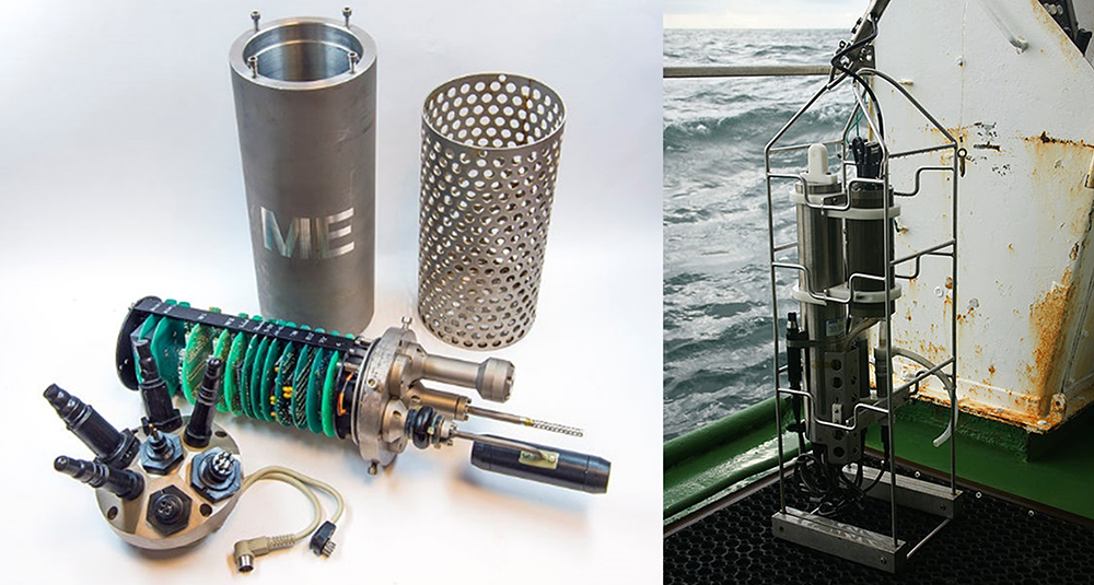
For more accurate measurements, most oceanographers use an instrument that measures electrical conductivity. An electrical current is passed between two electrodes immersed in water, and the higher the salinity, the more readily the current will be conducted (the ions in seawater conduct electrical currents). Conductivity probes are often bundled into an instrument called a CTD, which stands for Conductivity, Temperature, and Depth, which are the most commonly-measured parameters. Modern CTDs can be outfitted with an array of probes measuring parameters like light, turbidity (water clarity), dissolved gases etc. CTDs can be large instruments (below), but small hand-held salinity probes are also widely available.
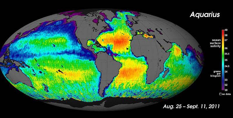
For large-scale salinity measurements, oceanographers can use satellites, such as the Aquarius satellite, which was able to measure surface salinity differences as small as 0.2 PSU as it mapped the ocean surface every seven days (below).
It is important to be aware that while the rule of constant proportions applies to most of the ocean, there may be certain coastal areas where lots of river discharge may alter these proportions slightly. Furthermore, it is important to remember that the rule of constant proportions only applies to the major ions. The proportions of the minor ions may fluctuate, but remember that they make a very minor contribution to overall salinity. Because the concentrations of the minor ions are not constant, these are referred to as non-conservative ions.
Why are the major ions found in constant proportions? There is constant input of ions from river runoff and other processes, usually in very different proportions from what is found in the ocean. So why don’t the proportions in the oceans change? Most of the ions discharged by rivers have fairly low residence times (see section 5.2) compared to ions in seawater, usually because they are used in biological processes. These low residence times do not allow the ions to accumulate and alter salinity. Also, the mixing time of the world ocean is around 1000 years, which is very short compared to the residence times of the major ions, which may be tens of millions of years long. So during the residence time of a single ion the ocean has mixed numerous times, and the major ions have become evenly distributed throughout the ocean.
Variations in Salinity
Total salinity in the open ocean averages 33-37 ppt, but it can vary significantly in different locations. But since the major ion proportions are constant, the regional salinity differences must be due more to water input and removal rather than the addition or removal of ions. Fresh water input comes through processes like precipitation, runoff from land, and melting ice. Fresh water removal primarily comes from evaporation and freezing (when seawater freezes, the resulting ice is mostly fresh water and the salts are excluded, making the remaining water even saltier). So differences in rates of precipitation, evaporation, river discharge, and ice formation play a significant role in regional salinity variations. For example, the Baltic Sea has a very low surface salinity of around 10 ppt, because it is a mostly enclosed body of water with lots of river input. Conversely, the Red Sea is very salty (around 40 ppt), due to the lack of precipitation and the hot environment which leads to high levels of evaporation.
One of the saltiest large bodies of water on Earth is the Dead Sea, between Israel and Jordan. Salinity in the Dead Sea is around 330 ppt, which is almost ten times saltier than the ocean. This extremely high salinity is a result of the hot, arid conditions in the Middle East that lead to high rates of evaporation. In addition, in the 1950s the flow from the Jordan River was diverted away from the Dead Sea, so there is no longer significant fresh water input. With no input and high evaporation, the water level in the Dead Sea is receding at a rate of about 1 m per year. The high salinity makes the water very dense, which creates buoyant forces that allow people to easily float at the surface. But the high salinity also means that the water is too salty for most living organisms, so only microbes are able to call it home; hence the name the Dead Sea. But as salty as the Dead Sea may be, it is not the saltiest body of water on Earth. That distinction currently belongs to Gaet’ale Pond in Ethiopia, with a salinity of 433 ppt!
Latitudinal Variations
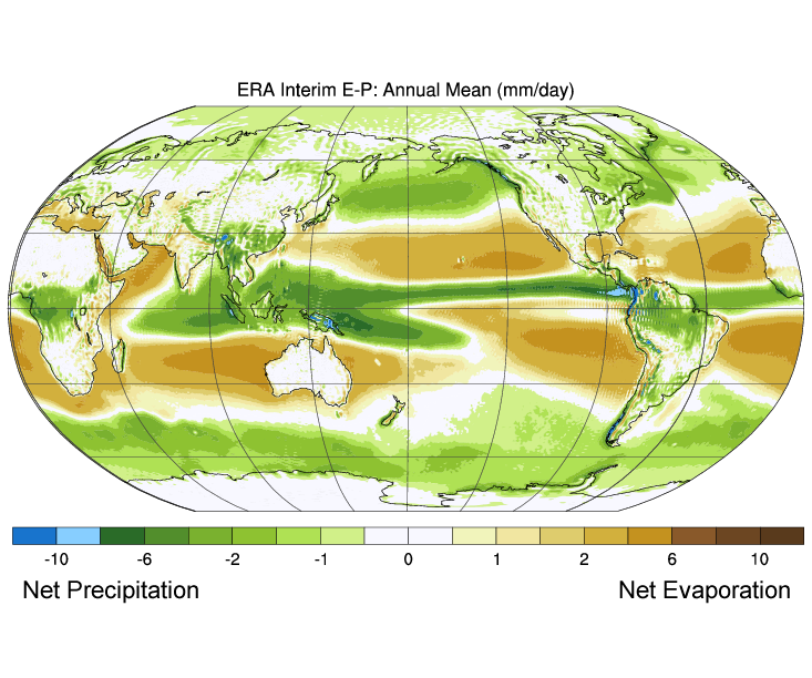
While local conditions are important for determining salinity patterns in any single location, there are some global patterns that bear further investigation. Temperature is highest at the equator, and lowest near the poles, so we would expect higher rates of evaporation, and therefore higher salinity, in equatorial regions (Figure 5.3.2). This is generally the case, but in the figure below salinity right along the equator seems to be a little lower than at slightly higher latitudes. This is because equatorial regions also get a high volume of rain on a regular basis, which dilutes the surface water along the equator. So the higher salinities are found at subtropical, warm latitudes with high evaporation and less precipitation. At the poles there is little evaporation, which, coupled with ice and snow melting, produces a relatively low surface salinity. The image below shows high salinity in the Mediterranean Sea; this is located in a warm region with high evaporation, and the sea is largely isolated from mixing with the rest of the North Atlantic water, leading to high salinity. Lower salinities, such as those around southeast Asia, are the result of precipitation and high volumes of river input.
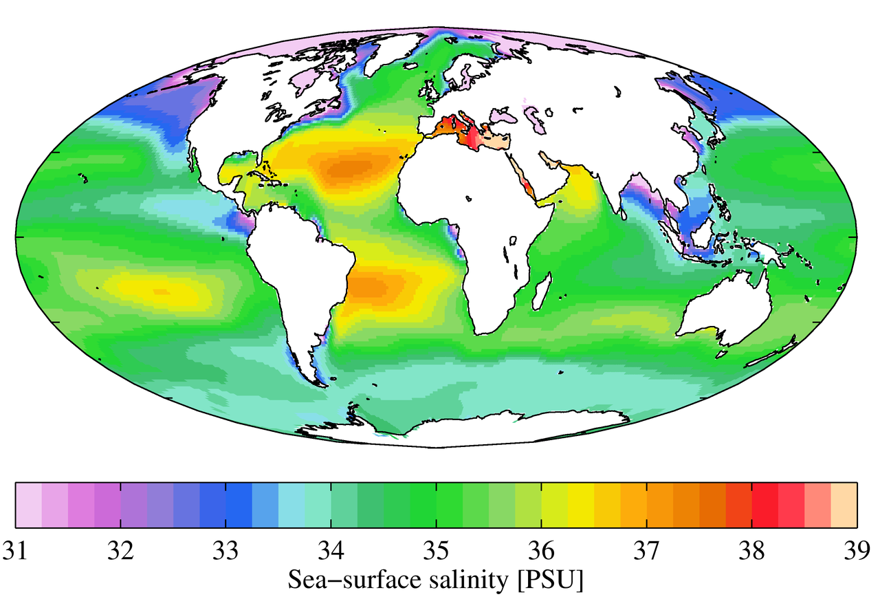
Figure 5.3.3 shows the mean global differences between evaporation and precipitation (evaporation – precipitation). Green colors represent areas where precipitation exceeds evaporation, while brown regions are where evaporation is greater than precipitations. Note the correlation between precipitation, evaporation, and surface salinity as seen in Figure 5.3.2.
Vertical Variation
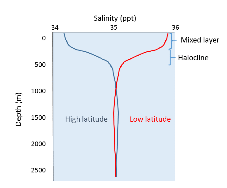
In addition to geographical variation in salinity, there are also changes in salinity with depth. As we have seen, most differences in salinity are due to variations in evaporation, precipitation, runoff, and ice cover. All of these process occur at the ocean surface, not at depth, so the most pronounced differences in salinity should be found in surface waters. Salinity in deeper water remains relatively uniform, as it is unaffected by these surface processes. Some representative salinity profiles are shown in Figure 5.3.4. At the surface, the top 200 m or so show relatively uniform salinity in what is called the mixed layer. Winds, waves, and surface currents stir up the surface water, causing a great deal of mixing in this layer and fairly uniform salinity conditions. Below the mixed layer is an area of rapid salinity change over a small change in depth. This zone of rapid change is called the halocline, and it represents a transition between the mixed layer and the deep ocean. Below the halocline, salinity may show little variation down to the seafloor, as this region is far removed from the surface processes that impact salinity. In the figure below, note the low surface salinity at high latitudes, and higher surface salinity at low latitudes as discussed above. Yet despite the surface differences, salinity at depth in both locations may be very similar.
an atom or molecule that has either gained or lost electrons and has thus become charged (5.1)
the concentration of dissolved ions in water (5.3)
a unitless measure of salinity equal to parts per thousand (5.3)
the six ions that comprise over 99% of the ions in the ocean (chloride, sodium, sulfate, magnesium, calcium, potassium) (5.3)
the major ions in seawater are always found in the same proportions, regardless of overall salinity (5.3)
ions whose proportions are the same regardless of overall salinity; the major ions in seawater (5.3)
ions in seawater whose proportions fluctuate with changes in salinity (5.3)
flow of water down a slope, either across the ground surface, or within a series of channels (12.2)
the average amount of time an element will remain in the ocean before being removed (5.2)
parts per thousand
the distance north or south of the equator, measured as an angle from the equator (2.1)
the topmost layer of the ocean, where winds, waves, and currents mix the water so that conditions are relatively constant; approximately the top 100 m (5.3)
where there is a dramatic change in salinity over a small change in depth (5.3)
