
9.8 Thermohaline Circulation
The surface currents we have discussed so far are ultimately driven by the wind, and since they only involve surface water they only affect about 10% of the ocean’s volume. However, there are other significant ocean currents that are independent of the wind, and involve water movements in the other 90% of the ocean. These currents are driven by differences in water density.
Recall that less dense water remains at the surface, while denser water sinks. Waters of different densities tend to stratify themselves into layers, with the densest, coldest water on the bottom and warmer, less dense water on top. It is the movement of these density layers that create the deep water circulation. Since seawater density depends mainly on temperature and salinity (section 6.3), this circulation is referred to as thermohaline circulation.
The main processes that increase seawater density are cooling, evaporation, and ice formation. Evaporation and ice formation cause an increase in density by removing fresh water, leaving the remaining seawater with greater salinity (see section 5.3). The main processes that decrease seawater density are heating, and dilution by fresh water through precipitation, ice melting, or fresh water runoff. Note that all of these processes exert their effects at the surface, but don’t necessarily affect deeper water. However, changing the density of the surface water causes it to sink or rise, and these vertical, density-driven movements create the deep ocean currents. These thermohaline currents are slow, on the order of 10-20 km per year compared with surface currents that move at several kilometers per hour.
Water masses
A water mass is a volume of seawater with a distinctive density as a result of its unique profile of temperature and salinity. As stated above, the processes that affect seawater density really only happen at the surface. Once a water mass has reached its particular temperature and salinity profile due to these surface processes, it may sink below the surface, at which point its density properties won’t really change. We can therefore distinguish particular water masses by taking salinity and temperature measurements at different depths, and looking for the unique combination of these variables that give it its characteristic density. This is often carried out using temperature-salinity diagrams (T-S diagrams, see box below).
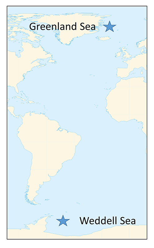
There are several well-known water masses in the ocean, particularly in the Atlantic, that are distinguished by their temperature and salinity characteristics. The densest ocean water is formed in two primary locations near the poles, where the water is very cold and highly saline as a result of ice formation. The densest deep water mass is formed in the Weddell Sea of Antarctica, and becomes the Antarctic Bottom Water (AABW). Similar processes in the North Atlantic produce the North Atlantic Deep Water (NADW) in the Greenland Sea (Figure 9.8.1).
This cold, dense water sinks, and once it is removed from the surface, its temperature and salinity remain unchanged, so it keeps the same characteristics as it moves throughout the ocean as part of the thermohaline circulation. AABW sinks to the bottom in the Weddell Sea and then moves north along the bottom into the Atlantic, and east through the Southern Ocean. At the same time NADW is sinking in the Greenland Sea. This water mass is less dense than AABW and tends to form a layer above the AABW as it flows across the equator to the south (Figure 9.8.2). As the NADW moves towards the Antarctic continent, it is brought to the surface. Recall that near Antarctica there is the Antarctic divergence, where surface waters move horizontally away from each other, and are replaced by deep water upwelling (bringing nutrients to the surface and leading to high productivity; see section 7.3). Since polar water has a weak thermocline, there isn’t much of a density difference preventing the deep water from reaching the surface, so some NADW rises as part of the upwelling process (Figure 9.8.2).
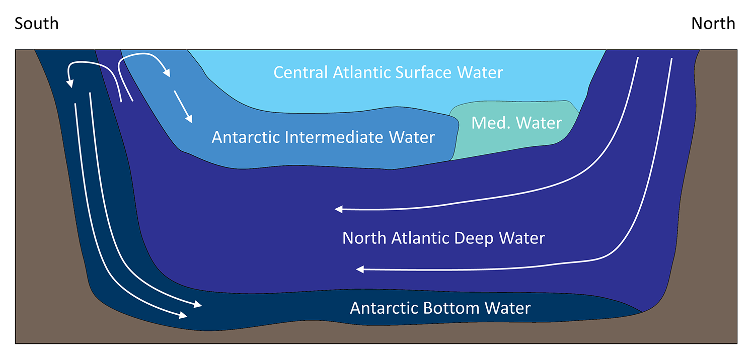
As the rising NADW reaches the surface, some travels south where it will eventually contribute to the production of new AABW. The NADW that moves north encounters the Antarctic convergence, which produces downwelling. This sinking NADW becomes a new water mass; Antarctic Intermediate Water (AAIW), which sinks and creates a layer between the surface water and the NADW (Figure 9.8.2). The surface water in the equatorial Atlantic, also called the Central Atlantic Surface Water, is very warm and low density, therefore it remains at the surface and does not contribute much to thermohaline circulation.
In the Atlantic, Mediterranean Intermediate Water (MIW) flows through the Straits of Gibraltar into the open ocean. This water is warm and salty from the warm temperatures and high evaporation characteristic of the Mediterranean Sea, so it is denser than the normal surface water and forms a layer about 1-1.5 km deep. Eventually this water will move north to the Greenland Sea, where it will be cooled and will sink, becoming the dense NADW.
T-S Diagrams
A temperature-salinity (T-S) diagram is used to examine how temperature, salinity, and density change with depth, and to identify the vertical structure of the water column, including the water masses it contains. Water temperature is on the y-axis, and salinity appears on the x-axis. Often, instead of the actual temperature of the water, oceanographers plot potential temperature, which is the temperature the water would achieve if it was brought to the surface and did not get any additional heat through compression at depth. A T-S diagram shows lines of equal density, or isopycnals, for various combinations of temperature and salinity (Figure 9.8.3). You can then plot the values of temperature and salinity on the diagram, and use their point of intersection to calculate the density of the water. In the example in Figure 9.8.3 a temperature of about 11o C and a salinity of 34.6 PSU results in a density of 1.0265 g/cm3.
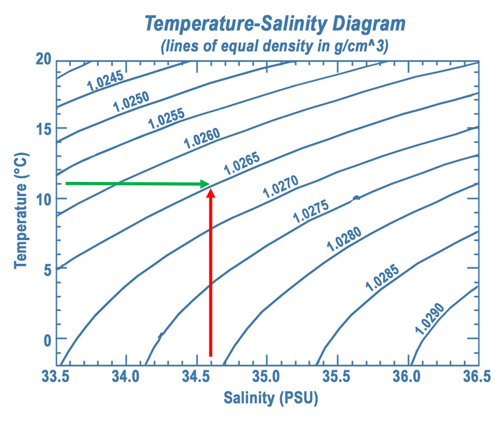
Since the range of densities in the ocean is rather small, often the density value is shortened and is expressed as sigma-t or σt. Sigma-t is calculated as: (density – 1) x 1000. So it essentially just looks at the last three decimal places of the density value. Thus a density of 1.0275 g/cm3 would have a σt of 27.5.
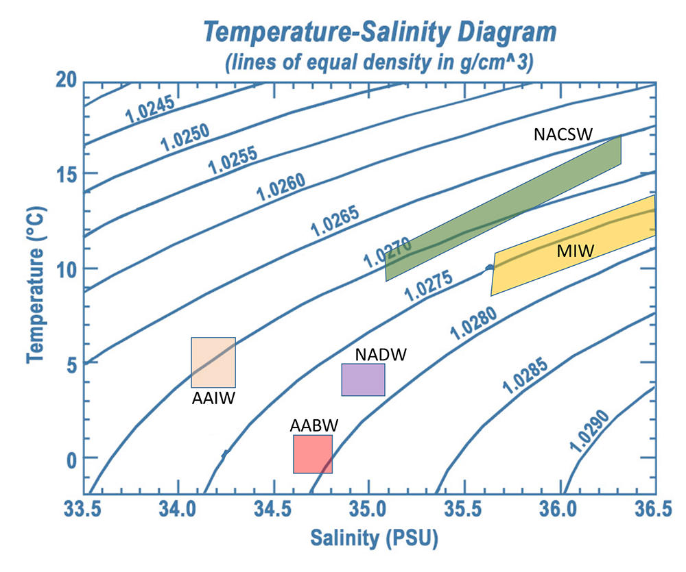
T-S diagrams can be used to identify water masses. Since each major water mass has its own characteristic range of temperatures and salinities, a deep water sample that falls into that range can presumably have come from that water mass. Figure 9.8.4 shows the typical range of temperature and salinity for the major Atlantic water masses.
To investigate water masses, oceanographers can take a series of temperature and salinity measurements over a range of depths at a particular location. If the water column was highly stratified and there was no mixing between or within the layers, as the probe was lowered your would get a series of constant temperature and salinity readings as you moved through the first water mass, followed by a sudden jump to another set of different but constant readings as you moved through the next water mass. Plotting temperature vs. salinity on a T-S diagram would result in a distinct and independent point for each water mass. However, in reality, the water masses will show some mixing within and between layers. So as the probes are lowered, they will encounter water that shows traits intermediate between the two points. Therefore, with increasing depth, the points on the T-S diagram will gradually move from one point to the other, creating a line connecting the two points, illustrating mixing between those two water masses.
In the example in Figure 9.8.5, NACSW is present at the surface (0 m depth), and between 0 and about 800 m there is a transition from NACSE into AAIW. Between about 800-2100 m there is a transition from AAIW into the NADW layer just beyond 2000 m. AABW is the deepest water mass, at depths of about 4000 m. The transition between NADW and AABW occurs between about 2100-4000 m.
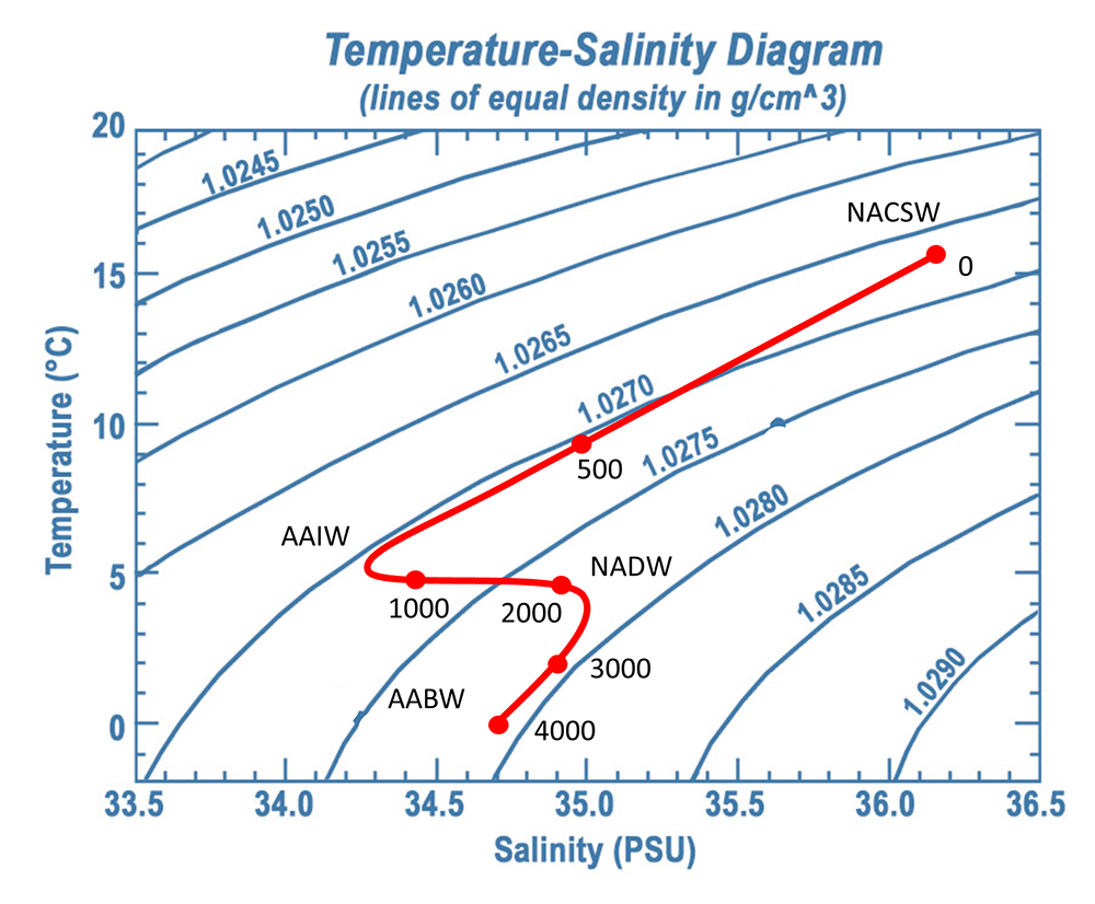
Notice that as the recordings get deeper in Figure 9.8.5, the density is always increasing (i.e. moving towards the bottom right corner). This is because the densest water should be located at the bottom, with the other layers stratified according to their density, otherwise the water column would be unstable.
The “Ocean Conveyor Belt”
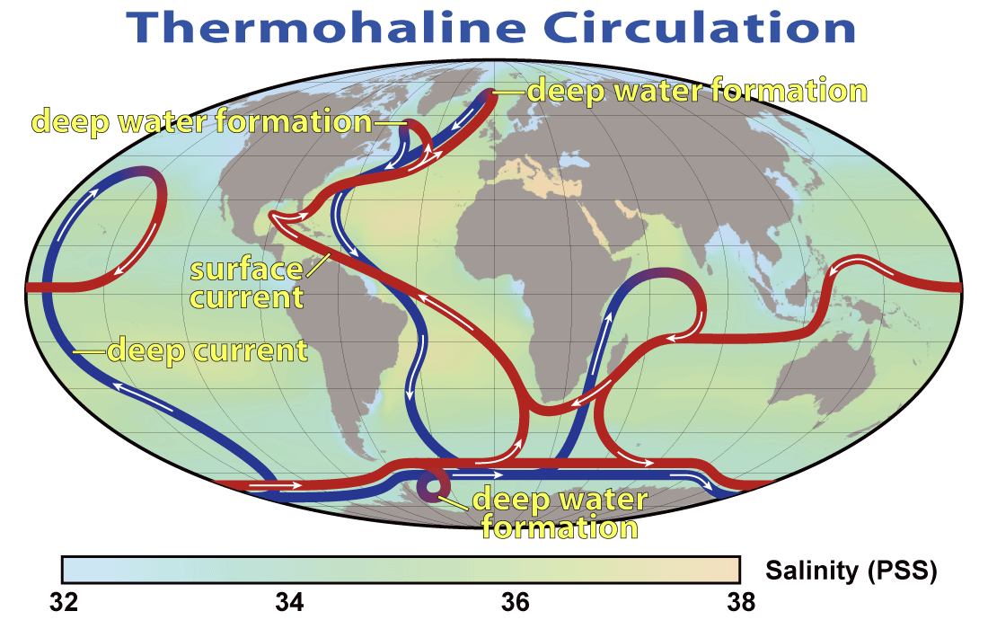
The bottom water from the Weddell Sea and Greenland Sea does not just circulate through the Atlantic. NADW moves south through the western Atlantic before meeting the AABW north of the Weddell Sea. Together these water masses move eastwards into the Indian and Pacific Oceans. By this time the NADW and AABW have started mixing, to create what is called Common Water. The deep Common Water moves northwards into the Pacific and Indian Oceans and gradually mixes with the warmer water, causing it to eventually rise to the surface. As surface water, it makes its way back to the North Atlantic through the surface currents of the Pacific and Indian Oceans. Once back in the North Atlantic, it cools and once again forms NADW, starting the process anew. This cycle of rising and sinking water transporting water between the surface and deep circulation has been referred to as the global oceanic “conveyor belt”, and may take about 1000-2000 years to complete (Figure 9.8.6).
This global circulation pattern has a number of important implications for Earth’s environment. For one, it is vital to the transport of heat around the globe, bringing warm water towards the poles, and cold water to the tropics, stabilizing temperature in both environments.
The conveyor belt also helps deliver oxygen to deep water habitats. The deep water began as cold surface water that was saturated with oxygen, and when it sank it brought that oxygen to depth. Thermohaline circulation carries this oxygen-rich deep water throughout the oceans, where the oxygen will be used by deep water organisms. Bottom water in the Atlantic is relatively high in oxygen, as it still retains much of its original oxygen content, but as it travels over the seafloor the oxygen is used up, so that deep water in the Pacific Ocean has much less oxygen than deep Atlantic water, with Indian Ocean water somewhere in between. At the same time, deep water will accumulate nutrients as organic matter sinks and decomposes. Atlantic bottom water is low in nutrients because it has not had much time to accumulate them, and the original surface water was nutrient-poor. By the time this bottom water reaches the Indian Ocean, and after that the Pacific, it has been accumulating the sinking nutrients for centuries, so deep nutrient concentrations are greater in the Pacific than the Atlantic. We can therefore use the ratios of oxygen to nutrients in the deep water to tell the relative age of a water mass, i.e. how long it has been since it sank from the surface. Younger bottom water should be high in oxygen and low in nutrients, while the opposite would be expected for older bottom water.
The ocean conveyor belt may be significantly impacted by climate change disrupting thermohaline circulation. Increased warming, particularly in the Arctic, could lead to continuing melting of the polar ice caps, adding a large amount of fresh water to the polar surface water. This input of fresh water could create a low density, low salinity surface layer of water that no longer sinks, thus disrupting the deep circulation conveyor belt and preventing oxygen and nutrient transport to bottom communities. The sinking of seawater in the Greenland Sea also helps drive the Gulf Stream; as water sinks, more surface water is pulled northwards in the Gulf Stream. If this polar water stops sinking the Gulf Stream could weaken, reducing heat transport to the poles and cooling the northern climate. It seems counter intuitive, but global warming could lead to colder conditions in Europe and the freezing of ports and cities that are usually ice-free due to the warming effects of the Gulf Stream. Recent evidence has already shown that the strength of the Gulf Stream is waning, likely due to the increased melting of Arctic ice.
mass per unit volume of a substance (e.g., g/cubic cm) (6.3)
the concentration of dissolved ions in water (5.3)
deep ocean circulation driven by differences in water density (9.8)
flow of water down a slope, either across the ground surface, or within a series of channels (12.2)
a volume of seawater with a distinctive density as a result of its unique profile of temperature and salinity (9.8)
process by which deeper water is brought to the surface (9.5)
in the context of primary production, substances required by photosynthetic organisms to undergo growth and reproduction (5.6)
the synthesis of organic compounds from aqueous carbon dioxide by plants, algae, and bacteria (7.1)
a region in the water column where there is a dramatic change in temperature over a small change in depth (6.2)
process by which surface water is forced downwards (9.5)
a unitless measure of salinity equal to parts per thousand (5.3)
the amount of a substance currently dissolved in the water, relative to the maximum possible content (5.4)
the major surface current flowing northwards along the Atlantic coast of the U.S. and Canada (9.2)
